Ecology Study Guide · BIOL 3340

U1 · The Nature of Ecology

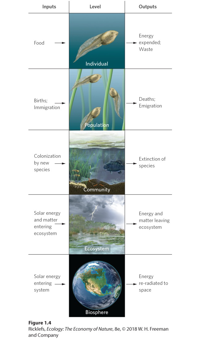
Ecology is the scientific study of the relationships between organisms and their environment, including both biotic (living) and abiotic (non-living) components. Organized at hierarchical scales: organism → population → community → ecosystem → biome → biosphere. The discipline is integrative, drawing on physiology, evolution, behavior, and earth sciences.

Levels of organization

Level	Definition	Example
Individual / Organism	One living thing, the unit of natural selection.	A single bison.
Population	Group of conspecifics in a defined area at one time.	Bison herd of Wind Cave NP.
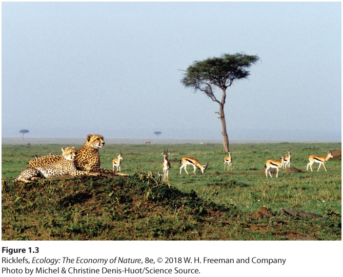
Community	All populations interacting in one place.	Tallgrass prairie community.
Ecosystem	Community + abiotic environment + energy/matter flow.	Glacier Creek Preserve.
Biome	Major regional vegetation type defined by climate.	Temperate grassland.
Biosphere	All life + its physical environment globally.	Earth's living envelope.

Doing ecology

Ecologists use observation, field experiments (manipulate variables in nature), laboratory experiments (high control, low realism), and modeling (quantitative predictions). Hypothesis testing relies on the scientific method, but ecology often deals in natural variation rather than controlled treatments.

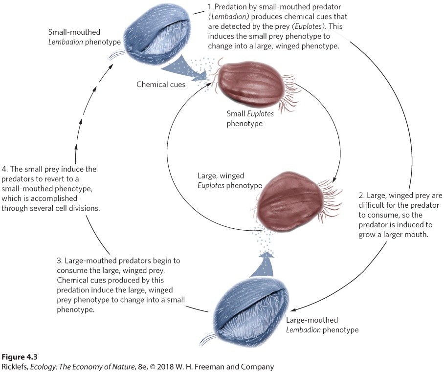
Adaptation = inherited trait that improves fitness in a given environment, produced by natural selection. Acclimation = reversible physiological change within a lifetime (e.g., fur thickening in winter). Plasticity = ability of one genotype to produce different phenotypes in different environments.

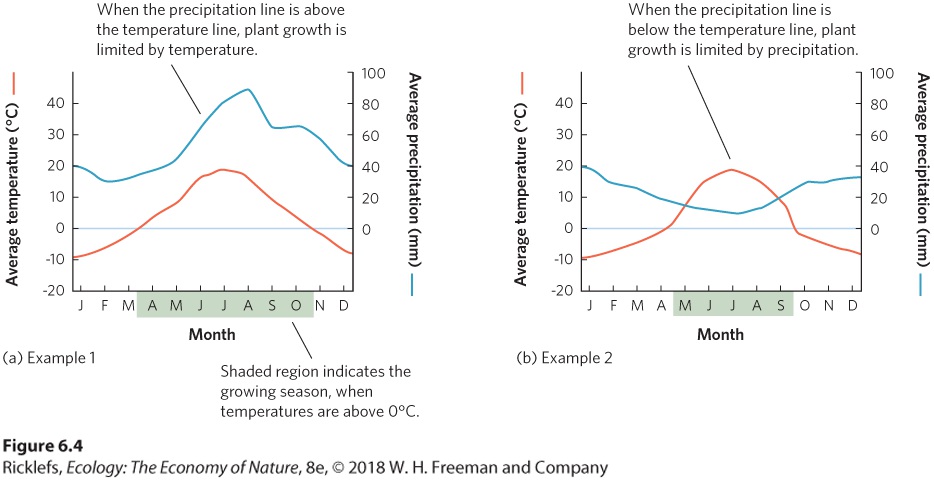
U2 · Climate

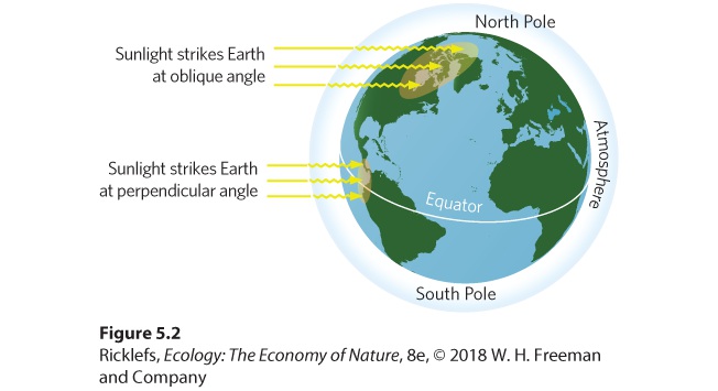
Hydrologic water cycle showing evaporation, transpiration, precipitation, runoff, infiltration — **Water cycle** — solar-driven evaporation + transpiration → atmospheric H₂O vapor → precipitation → runoff/infiltration → groundwater + surface flow back to ocean. *(Wikimedia Commons, public domain — USGS)*

Climate is the long-term average of weather. Driven by solar radiation, latitude (angle of incidence), and Earth's tilt (23.5°), giving us seasons.

Insolation: Incoming solar radiation per unit area, peaks at the equator, falls toward poles.
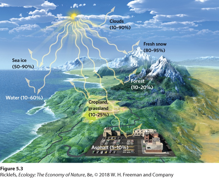
Albedo: Fraction of insolation reflected. Snow ~0.8, dark forest ~0.1.
Hadley cell: Atmospheric circulation: warm air rises at equator, sinks at ~30° latitude → tropical rainforests at equator, deserts at 30°.
Coriolis effect: Rotation deflects winds right in N. Hemisphere, left in S. → trade winds, westerlies.
Rain shadow: Air rises over a mountain, cools, drops rain on the windward side; descends dry on the leeward side.
El Niño / La Niña (ENSO): Periodic warming/cooling of equatorial Pacific that shifts global precipitation.
Microclimate: Small-scale climate variation due to topography, vegetation, or substrate; matters more to small organisms than regional climate.

Earth's energy budget

~30% of incoming solar radiation is reflected (albedo); ~70% absorbed. Re-radiated as longwave IR. Greenhouse gases (CO₂, CH₄, H₂O vapor) absorb that IR and warm the lower atmosphere — the greenhouse effect is what keeps Earth ~33 °C warmer than it would be otherwise.

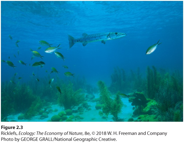
U3 · The Aquatic Environment

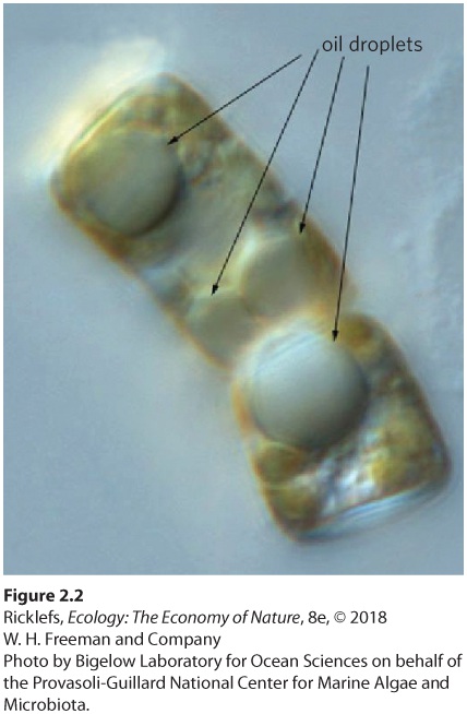
Water has unique properties critical for life: high specific heat, high heat of vaporization, density maximum at 4 °C, and ability to dissolve polar/ionic substances. Water is densest at 4 °C, so ice floats — protecting aquatic life beneath winter ice.

Lake stratification

Layer	Description
Epilimnion	Warm, well-mixed surface layer; high O₂, high light.
Thermocline (metalimnion)	Sharp temperature drop with depth — barrier to mixing.
Hypolimnion	Cold, dense bottom layer; low O₂, accumulates nutrients.

Spring + fall turnover: when surface water cools/warms to 4 °C, the layers equalize in density and wind mixes the lake top to bottom — bringing nutrients up + oxygen down.

Oligotrophic: Nutrient-poor, deep, clear, cold lake (e.g., Crater Lake).
Eutrophic: Nutrient-rich, shallow, warm, often algal-bloom-prone lake.
Lotic vs lentic: Flowing (rivers, streams) vs still (lakes, ponds) freshwater systems.
Salinity: Dissolved salts; freshwater <0.5 ppt, brackish 0.5–30 ppt, marine 30–37 ppt.
Estuary: Where freshwater rivers meet the sea — productive, salinity gradient.

Ocean chemistry

The carbonate buffer system (CO₂ + H₂O ⇌ H₂CO₃ ⇌ HCO₃⁻ + H⁺ ⇌ CO₃²⁻ + 2H⁺) keeps seawater near pH 8.1. Rising atmospheric CO₂ → ocean acidification → lower carbonate ion availability → harder for corals and shellfish to build CaCO₃ shells.

U4 · The Terrestrial Environment

Soil = mineral particles + organic matter + water + air + living organisms. Forms over thousands of years from weathering of bedrock by physical, chemical, and biological agents.

Soil horizons: O (organic litter) → A (topsoil, dark, humic) → E (eluviated, leached) → B (subsoil, accumulation) → C (parent material) → R (bedrock).
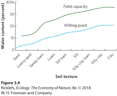
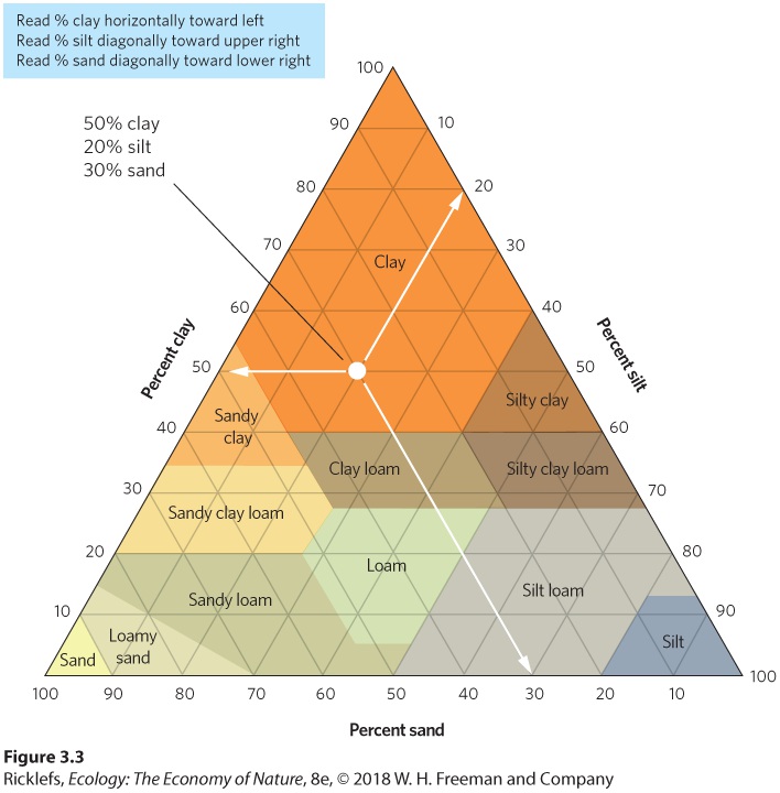
Soil texture: Relative % of sand / silt / clay. Loam = best balance for water + air + nutrients.
Cation exchange capacity (CEC): Ability of soil particles (esp. clay + humus) to hold cations like Ca²⁺, K⁺, NH₄⁺ for plant uptake.
Field capacity: Water held in soil after gravity drainage — available to plants.
Wilting point: Soil moisture below which plants cannot extract water.
Five soil-forming factors: Climate, organisms, relief (topography), parent material, time (Jenny's CLORPT).

U5 · Plant & Animal Adaptations

Plant adaptations

Photosynthesis pathway	Where	Trade-off
C3	Most temperate plants	Cool/wet conditions; loses CO₂ to photorespiration in heat.
C4	Tropical grasses, corn, sugarcane	Concentrates CO₂ with PEP carboxylase → efficient in hot/sunny.
CAM	Succulents (cacti, agave)	Stomata open at night → minimal water loss in deserts.

Animal thermal strategies

Ectotherm: Body T set by environment (reptiles, fish). Low metabolic cost; behavior-based thermoregulation.
Endotherm: Generates heat metabolically (mammals, birds). High food cost; constant body T.
Heterotherm: Switches modes — bats, hummingbirds (torpor); ground squirrels (hibernation).
Bergmann's rule: Endotherms tend to be larger in colder climates (lower SA:V → less heat loss).
Allen's rule: Appendages tend to be shorter in colder climates (less SA for heat loss).
Countercurrent heat exchange: Arteries and veins run antiparallel → heat transferred back to body before reaching cold extremities.

U6 · Population Properties & Growth

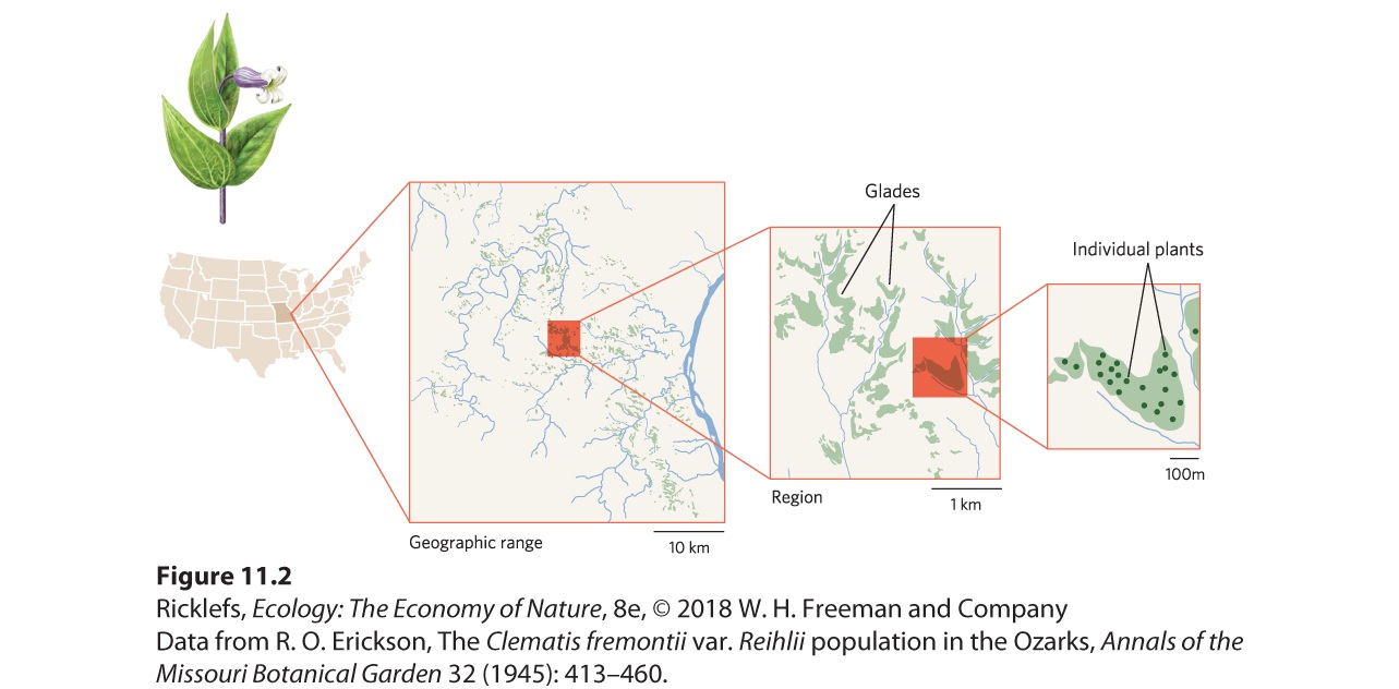
Logistic growth curve approaching carrying capacity K — **Logistic growth** — dN/dt = rN(1−N/K). Population grows exponentially when small, slows as it approaches carrying capacity K, levels off at K. Density-dependent regulation. *(Wikimedia Commons, public domain)*

Population density: Number of individuals per unit area / volume.
Dispersion: Pattern of spacing: uniform (territorial), random (rare in nature), clumped (most common — patchy resources).
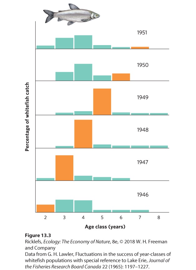
Survivorship curves: Type I high juvenile survival, mortality late (humans, elephants); Type II constant mortality (birds, small mammals); Type III high juvenile mortality (fish, plants).
Cohort vs static life table: Cohort follows one birth group through life; static is a snapshot of all ages now.
Net reproductive rate (R₀): Average number of offspring per female per generation. R₀ = 1 → stable.

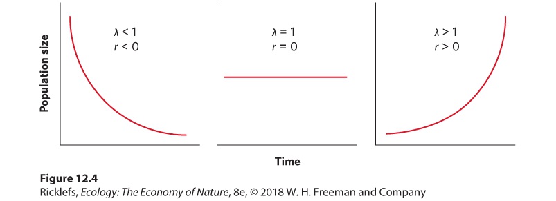
Population growth models

Exponential growth: dN/dt = rN. Unlimited resources → J-shaped curve.
Logistic growth: dN/dt = rN(1 − N/K). Resource-limited → S-shaped curve approaching carrying capacity (K).

Strategy	r-selected	K-selected
Body size	Small	Large
Lifespan	Short	Long
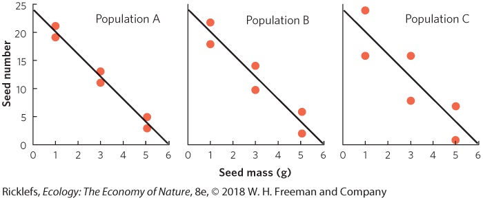
Reproduction	Many, small offspring; once or early	Few, large offspring; repeated
Habitat	Disturbed, unpredictable	Stable, predictable
Examples	Insects, dandelions	Whales, oaks

U7 · Population Regulation & Life History

Density-dependent factors: Effects intensify as N rises: competition, disease, predation. Stabilize populations.
Density-independent factors: Effects don't scale with N: weather, fire, floods. Cause crashes regardless of density.
Allee effect: Per-capita growth rate decreases at very low densities (mate finding, group defense fails).
Metapopulation: Set of local populations connected by dispersal. Source-sink dynamics: source populations have surplus dispersers; sink populations need immigration to persist.
Semelparity: One reproductive event then die (salmon, agave).
Iteroparity: Multiple reproductive events over a lifetime (most mammals).

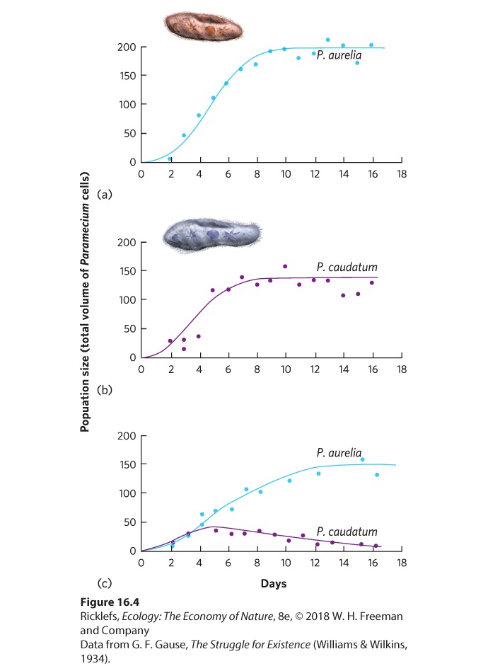
U8 · Competition

Intraspecific competition — among members of the same species — is the strongest form because resource needs overlap completely. Interspecific competition involves two or more species competing for shared resources.

Exploitation competition: Indirect — one consumer reduces the resource available to another.
Interference competition: Direct — aggression, allelopathy, territoriality.
Competitive exclusion principle (Gause): Two species with identical niches cannot coexist; one will outcompete the other.
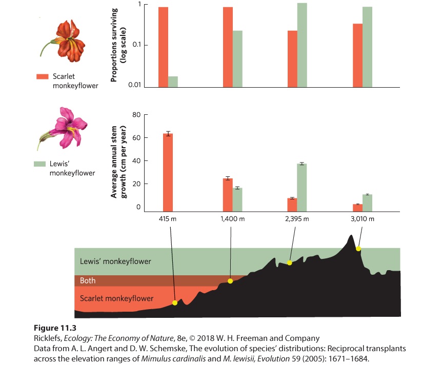
Fundamental niche: Full range of conditions a species can tolerate without competition.
Realized niche: Niche actually occupied after competition (subset of fundamental).
Resource partitioning: Species divide resources by time, space, or type (e.g., MacArthur's warblers feeding in different parts of spruce trees).
Character displacement: Trait differences exaggerated in sympatry (where species overlap) reducing competition.

Lotka-Volterra competition equations

dN₁/dt = r₁N₁(K₁ − N₁ − α₁₂N₂)/K₁
dN₂/dt = r₂N₂(K₂ − N₂ − α₂₁N₁)/K₂

α_ij = competition coefficient (effect of species j on species i). Coexistence requires each species to limit itself more than it limits the other.

U9 · Predation, Herbivory, Parasitism

Functional response: Predator's per-capita kill rate vs prey density. Type I linear; Type II saturating (handling time); Type III sigmoidal (prey switching).
Numerical response: Predator population growth in response to prey abundance.
Optimal foraging theory: Foragers maximize energy gained per unit time, balancing search and handling.
Predator-prey cycles: Lotka-Volterra: prey peak → predator peak (lag) → prey crash → predator crash (lag). Classic example: lynx + snowshoe hare 10-year cycle.
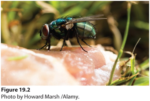
Aposematism: Warning coloration of toxic prey (monarch butterfly).
Batesian mimicry: Edible mimic of toxic model (viceroy butterfly).
Müllerian mimicry: Multiple toxic species converge on similar warning signals (Heliconius butterflies).
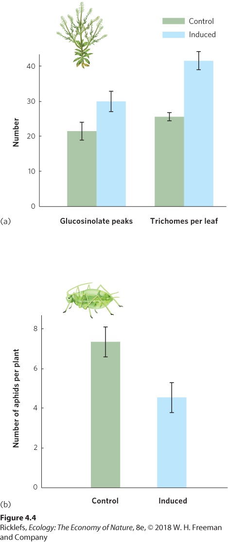
Plant chemical defenses: Tannins, alkaloids, glucosinolates — induced or constitutive.
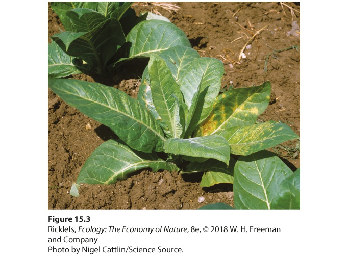
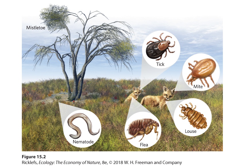
Parasitism: + / − interaction; parasite benefits at host's expense without (immediately) killing.
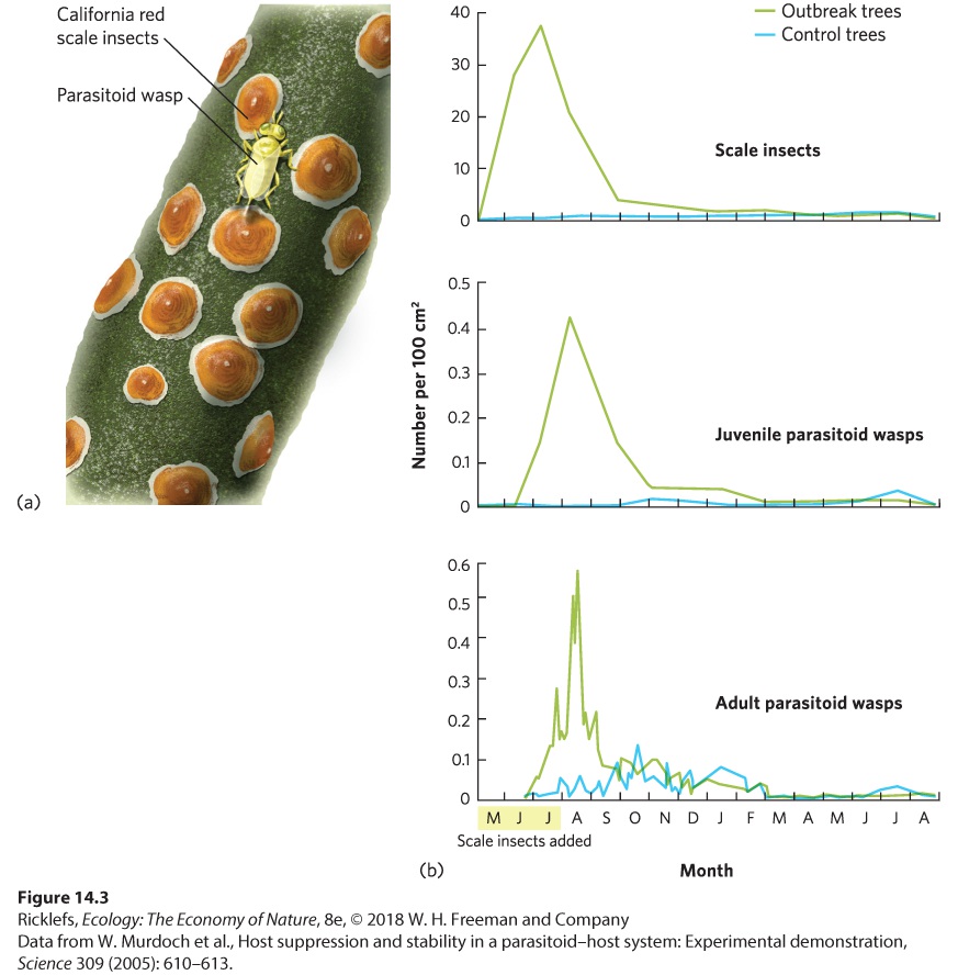
Parasitoid: Lays eggs in/on host; larvae kill host (parasitic wasps).

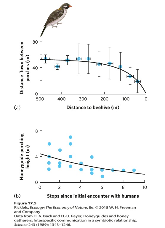
U10 · Mutualism & Coevolution

Mutualism: +/+ interaction. Obligate (one or both can't survive alone) or facultative.
Commensalism: +/0 (one benefits, other unaffected) — very rare; most "commensals" turn out subtly costly.
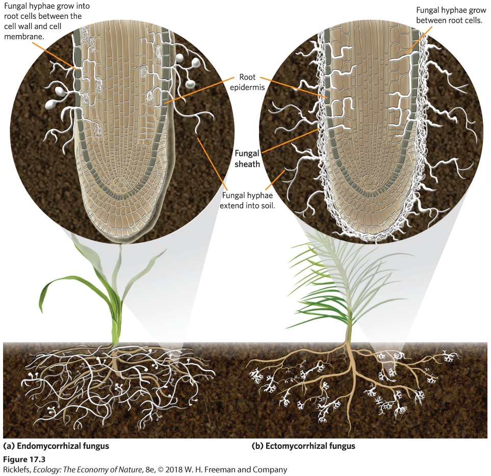
Mycorrhizae: Fungi-root mutualism. Arbuscular (endomycorrhizal) fungi penetrate root cortex (~80% plants); Ectomycorrhizal fungi sheath roots (mostly trees).
Pollination syndrome: Flower traits matched to pollinator: bee (UV pattern, sweet scent), hummingbird (red, tubular), bat (white, night-opening, musky), wind (no petals).
Coevolution: Reciprocal evolutionary change between interacting species (predator-prey, host-parasite, plant-pollinator).
Coral-zooxanthellae: Photosynthetic dinoflagellates inside coral cells provide ~90% coral energy. Stress → bleaching (loss of zoox).
Gut symbionts: Termite gut protists digest cellulose; ruminant rumen bacteria ferment plant material.

U11 · Community Structure & Diversity

Simple food web showing producers, primary consumers, secondary consumers — **Food web** — producers (plants/phytoplankton) → primary consumers (herbivores) → secondary consumers (carnivores) → top predators · decomposers recycle organic matter. *(Wikimedia Commons, public domain)*

Species richness (S): Number of species present.
Species evenness: How equally abundance is distributed across species.
Shannon-Wiener index (H'): H' = −Σ p_i ln(p_i); combines richness + evenness.
Simpson's index: Probability that two randomly drawn individuals are different species.
α / β / γ diversity: α = within-site; β = turnover between sites; γ = total regional. γ = α × β (approx).
Rank-abundance curve: Plot of log abundance vs species rank; steeper slope = lower evenness.
Dominant species: Most abundant or highest biomass; may not control community.
Keystone species: Disproportionate effect relative to abundance (e.g., Pisaster sea star — Paine's classic experiment).
Ecosystem engineer: Modifies habitat physically (beavers, prairie dogs, corals).
Food web: Network of feeding relationships. Bottom-up control = primary producers limit higher trophic levels; top-down = predators control prey, cascading down (trophic cascade).

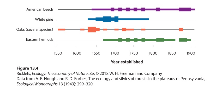
U12 · Succession & Disturbance — Bragg specialty

Succession = directional, predictable change in community composition over time following disturbance.

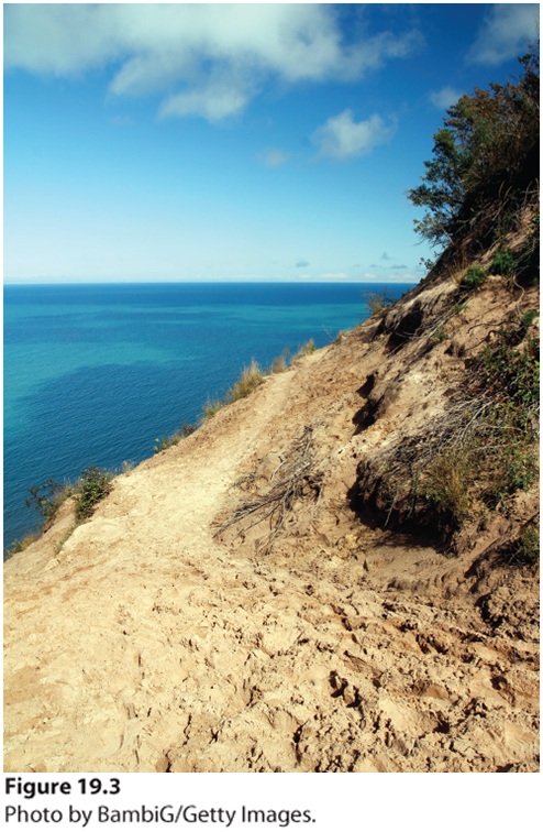
Primary succession: On bare substrate with no soil (volcanic flow, glacial retreat, sand dunes). Slow — pioneers like lichens build soil.
Secondary succession: Soil intact, propagules present (after fire, agriculture, logging). Faster.
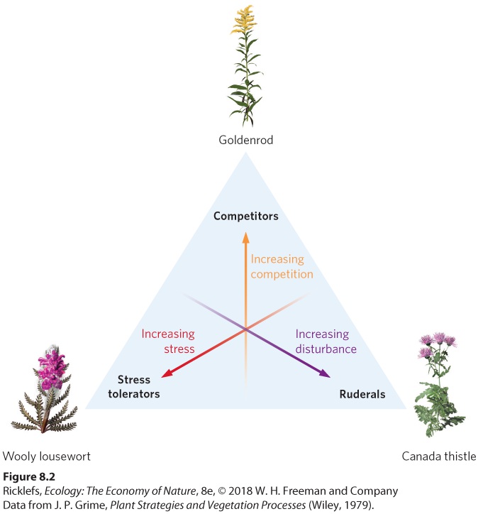
Pioneer species: Early colonizers — fast growth, wind-dispersed, stress-tolerant (e.g., fireweed, lichens).
Climax community: Theoretical end-state in stable equilibrium — challenged by modern non-equilibrium thinking.
Facilitation: Earlier species make conditions better for later (alder fixes N → spruce can grow).
Inhibition: Earlier species prevent later from establishing.
Tolerance: Later species establish despite earlier — depends on tolerating low light/nutrients.
Intermediate Disturbance Hypothesis (IDH): Diversity peaks at moderate disturbance frequency/intensity. Too little = competitive exclusion; too much = only ruderals survive.

Fire ecology — Bragg's research focus

Fire regime: Characteristic frequency, intensity, season, and patchiness of fire in an ecosystem.
Crown fire vs surface fire: Crown burns canopy (catastrophic, conifers); surface burns understory + litter (typical of grasslands).
Pyrogenic species: Adapted to or dependent on fire: serotinous cones (jack pine, lodgepole pine open only after fire), thick bark (oak, ponderosa pine), basal sprouting.
Tallgrass prairie: Maintained by frequent fire (~3–5 yr return). Fire suppresses woody invasion, recycles nutrients, stimulates C4 grass productivity.
Fire return interval: Years between fires at a site.
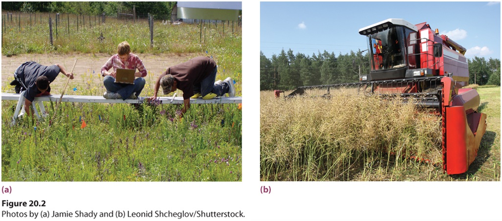
Prescribed burning: Management tool. Bragg's research at Glacier Creek Preserve tests season + frequency effects on prairie composition.
Loess Hills prairie: Western Iowa wind-deposited silt prairie — fire-dependent, threatened.

U13 · Ecosystem Energy & Nutrient Cycling

Ecological pyramid showing energy transfer between trophic levels — **Trophic pyramid** — only ~10% of energy passes between trophic levels (Lindeman's 10% rule). Producers form base · top carnivores at apex. Limits chain length to 4–5 levels. *(Wikimedia Commons, CC-BY-SA)*

Global carbon cycle showing reservoirs and fluxes — **Carbon cycle** — atmospheric CO₂ ↔ photosynthesis/respiration ↔ biomass · ocean DIC reservoir · long-term: weathering, sediments, fossil fuels. Anthropogenic CO₂ disrupts the balance. *(Wikimedia Commons, public domain)*

Nitrogen cycle showing fixation, nitrification, denitrification, ammonification — **Nitrogen cycle** — N₂ fixation (Rhizobium, cyanobacteria) → NH₄⁺ → NO₂⁻ → NO₃⁻ (nitrification) → plant uptake → ammonification → denitrification (NO₃⁻ → N₂) closes the loop. *(Wikimedia Commons, CC-BY-SA)*

Gross primary productivity (GPP): Total photosynthesis per unit time per area.
Net primary productivity (NPP): GPP − plant respiration. Energy available to consumers.
Trophic level: Position in food chain: producers (1°), primary consumers (2°), etc.
10% rule: Only ~10% of energy at one trophic level is incorporated into the next; rest lost as heat (2nd law). Limits chain length to ~4–5 levels.
Eltonian pyramid: Pyramid of energy, biomass, or numbers — energy always pyramidal; biomass occasionally inverted (open ocean — fast turnover phytoplankton).
Detritus food chain: Decomposers + detritivores process dead matter — often >50% of community energy flow.

Biogeochemical cycles

Cycle	Atmospheric pool?	Key fluxes
Carbon	Yes (CO₂)	Photosynthesis ↔ respiration; combustion of fossil fuels adds.
Nitrogen	Yes (N₂, ~78%)	N-fixation (Rhizobium, lightning, Haber-Bosch) → ammonification → nitrification (NH₄⁺→NO₂⁻→NO₃⁻) → denitrification (NO₃⁻→N₂).
Phosphorus	NO atmospheric pool	Weathering of rock → soil → plants → animals → return via decomposition. Often limiting.
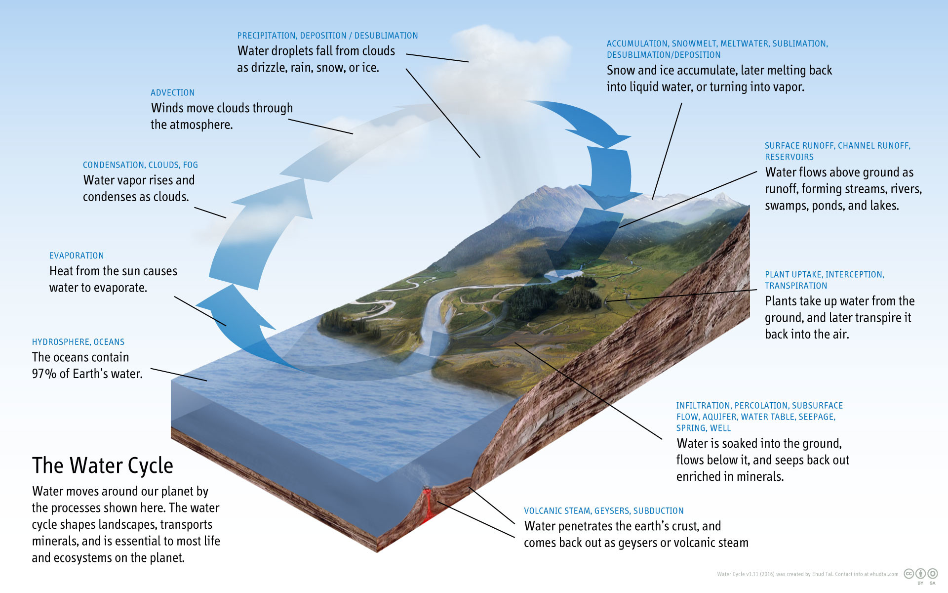
Water	Yes (vapor)	Evaporation, transpiration, precipitation, runoff. Solar-driven.

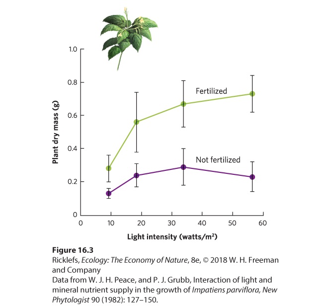
Limiting nutrient: Element that constrains productivity. Liebig's Law of the Minimum.
Eutrophication: Nutrient enrichment (often N, P from fertilizer runoff) → algal bloom → death + decomposition → hypoxic dead zone.
Bioaccumulation / biomagnification: Persistent pollutants (DDT, mercury) concentrate up food chains; top predators get hit hardest.

U14 · Biomes, Biogeography, Conservation

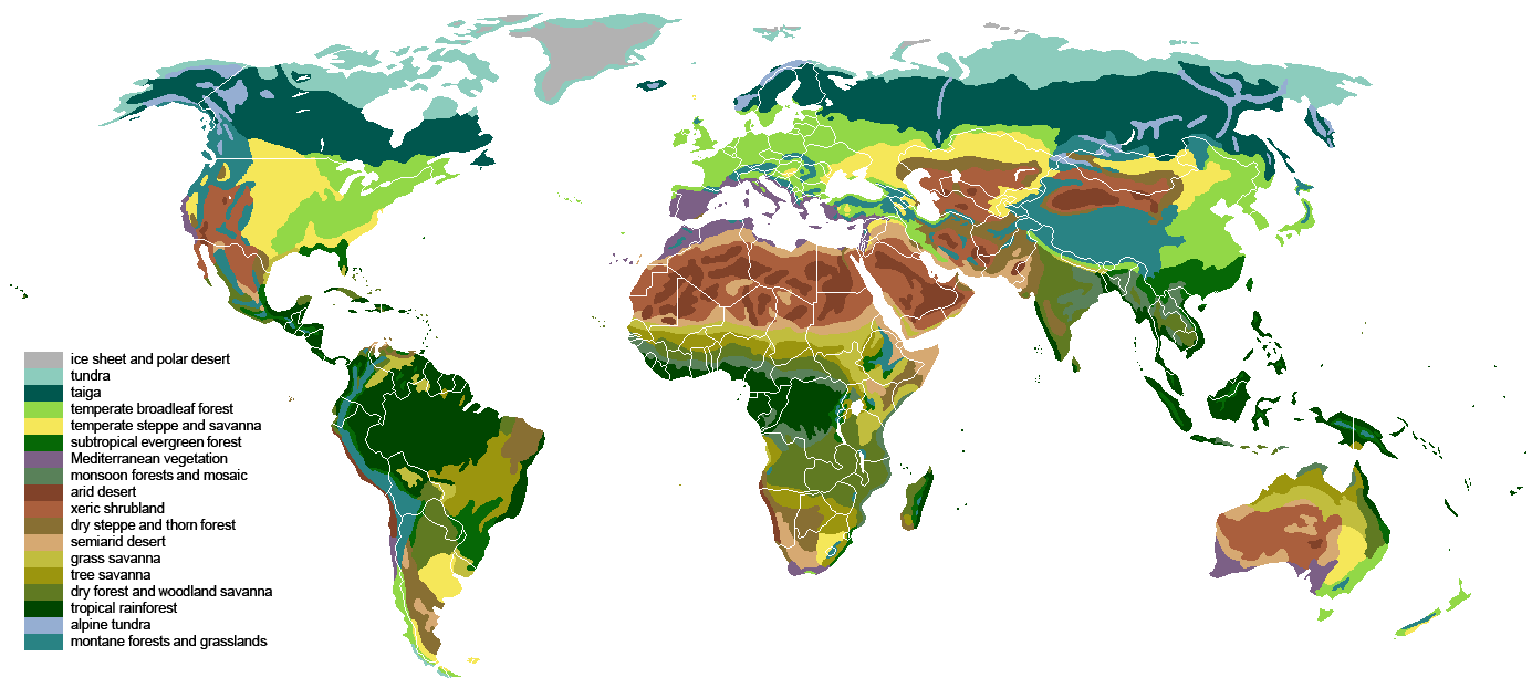
World vegetation map showing global biomes — **Global biome distribution** — climate (temperature × precipitation) defines biome zones. Tropics: rainforest, savanna · temperate: deciduous forest, grassland · boreal: taiga · polar: tundra · arid: desert. *(Wikimedia Commons, public domain)*

Major biomes (climate-defined)

Biome	Climate	Notes
Tropical rainforest	Warm, wet year-round	Highest biodiversity, low-fertility soils.
Tropical savanna	Warm, seasonal rain	Grass + scattered trees; fire-maintained.
Desert	Low precipitation	Hot or cold; CAM plants, ectotherms.
Temperate grassland	Hot summer, cold winter, moderate rain	Tallgrass prairie (Nebraska!), shortgrass steppe — fire-maintained.
Temperate deciduous forest	4 seasons, ~75-150 cm rain	Eastern US — oak, hickory, maple.
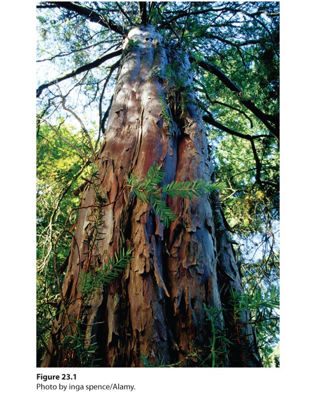
Boreal forest (taiga)	Long cold winter	Conifers — spruce, fir, pine.
Tundra	Permafrost, short growing season	Mosses, lichens, dwarf shrubs.
Mediterranean (chaparral)	Hot dry summer, mild wet winter	California, Mediterranean basin; fire-maintained.

Biogeography & conservation

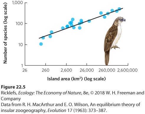
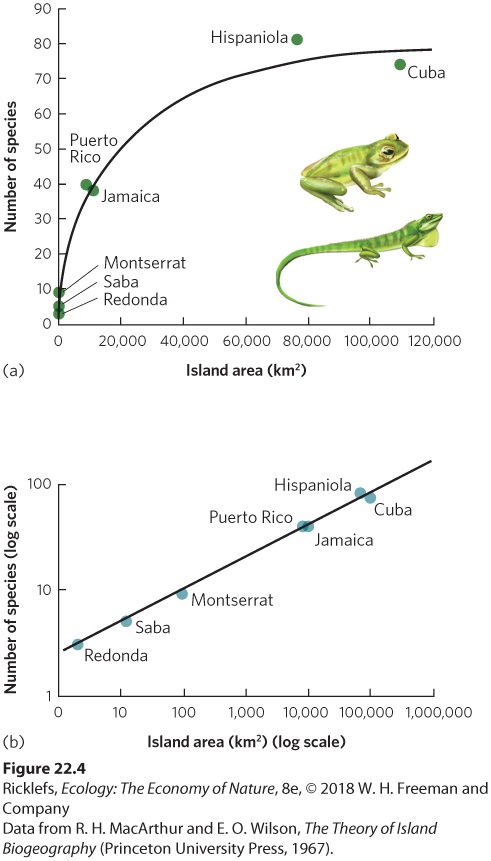
Island biogeography (MacArthur & Wilson): Species number on island = balance of immigration (decreases with distance to mainland) and extinction (decreases with island area). Larger + closer = more species.
Species-area relationship: S = cA^z. Doubling area roughly increases S by 10-25%.
Habitat fragmentation: Continuous habitat broken into smaller patches → edge effects, reduced gene flow, smaller populations.
Edge effect: Different conditions at habitat boundaries — wind, light, predators penetrate.
Minimum viable population (MVP): Smallest population likely to persist (~95% probability) for some interval (often 100 years).
Restoration ecology: Active reassembly of degraded ecosystems. Bragg's prairie burning experiments inform tallgrass restoration.
Biodiversity hotspot: Region with high endemism + high threat (Myers et al.).
Sixth extinction: Current human-driven mass extinction; rate ~100–1000× background.

Bragg-targeted exam tips

Know the tallgrass prairie and Loess Hills systems cold — locations, dominant species, fire regime.
Be ready for fire ecology mechanisms: pyrogenic adaptations, fire-return interval effects, woody encroachment when fire is suppressed.
Bring this site's printable cheat sheet on exam day — Bragg allows any materials.
Photo-rich slide questions: review his lecture images on Canvas (he photographed many himself).