Ch 1Introduction: Ecology, Evolution, and the Scientific MethodRead full chapter →
1Introduction: Ecology, Evolution, and the Scientific Method A deep-sea vent. In some regions of the ocean floor, hot water containing sulfur compounds is released from the ground. The sulfur compounds provide energy for chemosynthetic bacteria, which then serve as food for many other species that live near the vents, including these rust-colored tube worms (Tevnia jerichonana) that have been stained orange by iron compounds emitted from the vents. Searching for Life at the Bottom of the Ocean In the early 1800s, scientists hypothesized that deep ocean waters— depths greater than 275 m where s…
Sections in this chapter
- Searching for Life at the Bottom of the Ocean
- Learning Objectives
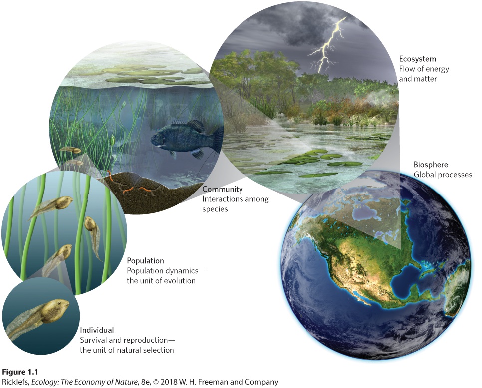
- 1.1 Ecological Systems Exist in a Hierarchy of Organization
- Individuals
- Populations and Species
- Communities
- Ecosystems
- The Biosphere
- Organization
- Concept Check
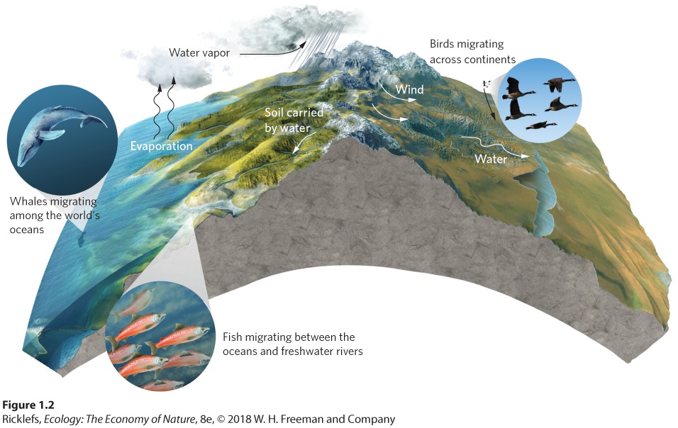
- 1.2 Ecological Systems Are Governed by Physical and Biological Principles
- Conservation of Matter and Energy
Ch 2Adaptations to Aquatic EnvironmentsRead full chapter →
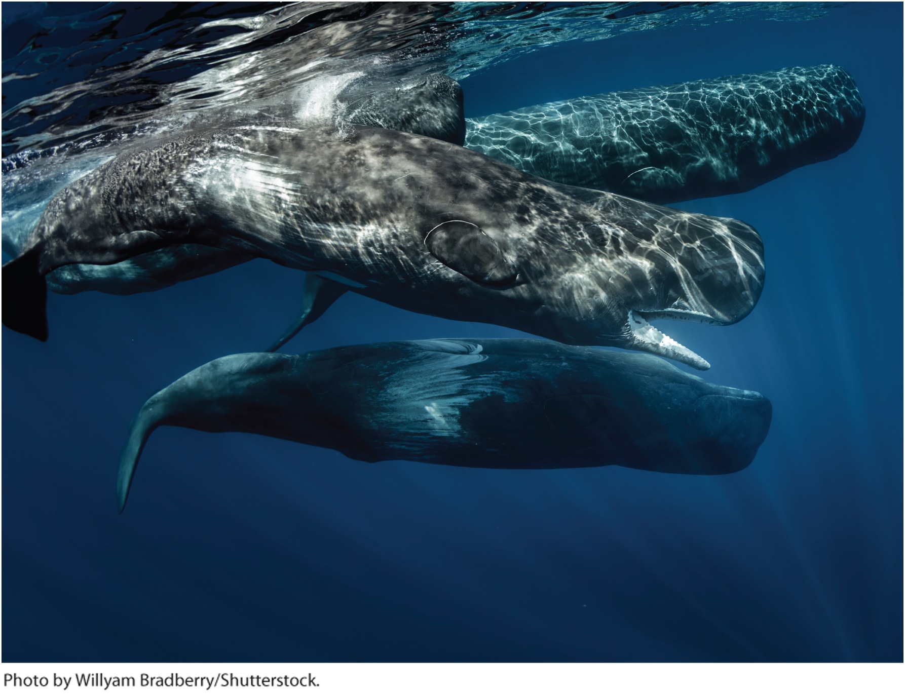
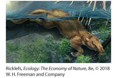
2Adaptations to Aquatic Environments Sperm whale. Modern whales, such as these sperm whales (Physeter macrocephalus) swimming off the coast of Portugal, have a number of adaptations that enable them to live in an aquatic environment. The Evolution of Whales Life on Earth began in the water. Of the many species that live in water, some of the most fascinating are the whales—a group that is particularly well suited to aquatic life. Surprisingly, the ancestor of modern whales can be traced back to a terrestrial mammal related to cattle, pigs, and hippos. Scientists first proposed an evolutionary …
Sections in this chapter
- 2 Adaptations to Aquatic Environments
- Learning Objectives
- Thermal Properties of Water
- Density and Viscosity of Water
- Dissolved Inorganic Nutrients
- Concept Check
- The Challenge of Salt and Water Balance
- Adaptations for Osmoregulation in Freshwater
- Adaptations for Osmoregulation in Saltwater
- Adaptations for Osmoregulation in Aquatic Plants
- Analyzing Ecology
- Carbon Dioxide
Ch 3Adaptations to Terrestrial EnvironmentsRead full chapter →
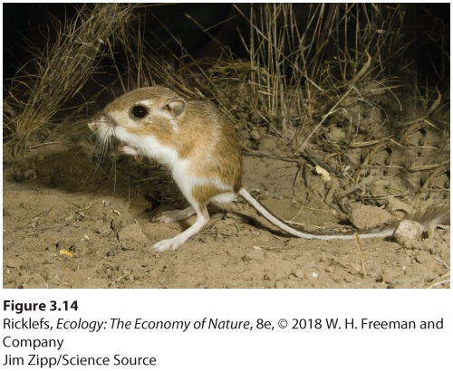
3Adaptations to Terrestrial Environments Adaptations of the dromedary camel. Dromedary camels, such as this one in the Hajar Mountains of the United Arab Emirates, have a wide range of adaptations that allow them to live in hot, dry environments. The Evolution of Camels When you think of camels, you might envision the iconic animals of the African and Asian deserts. The ancestor of all camel species actually originated in North America about 30 million years ago and camels roamed many parts of North America until about 8,000 years ago. Current evidence suggests that some of these ancestors cro…
Sections in this chapter
- 3 Adaptations to Terrestrial Environments
- Learning Objectives
- Soil Nutrients
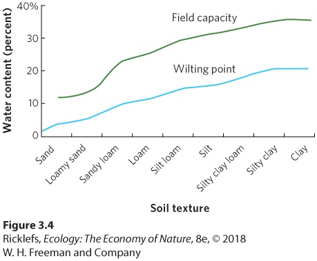
- Soil Structure and Water-Holding Capacity
- Osmotic Pressure and Water Uptake
- Concept Check
- Available and Absorbed Solar Energy
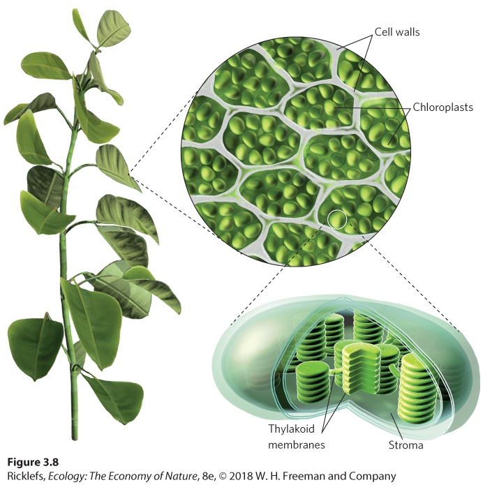
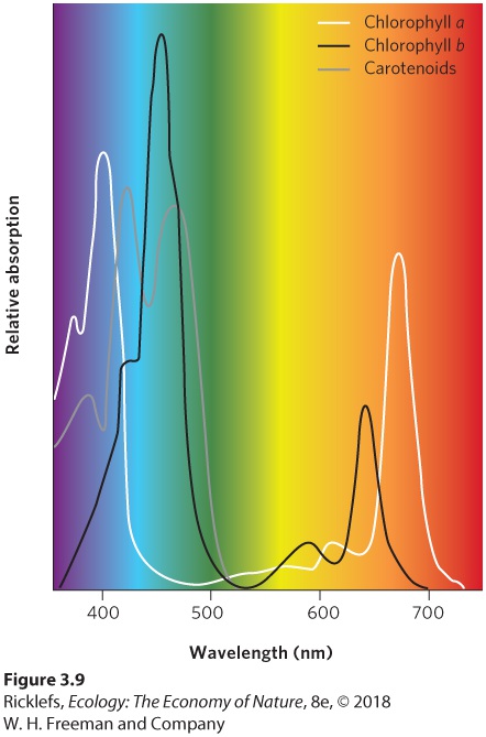
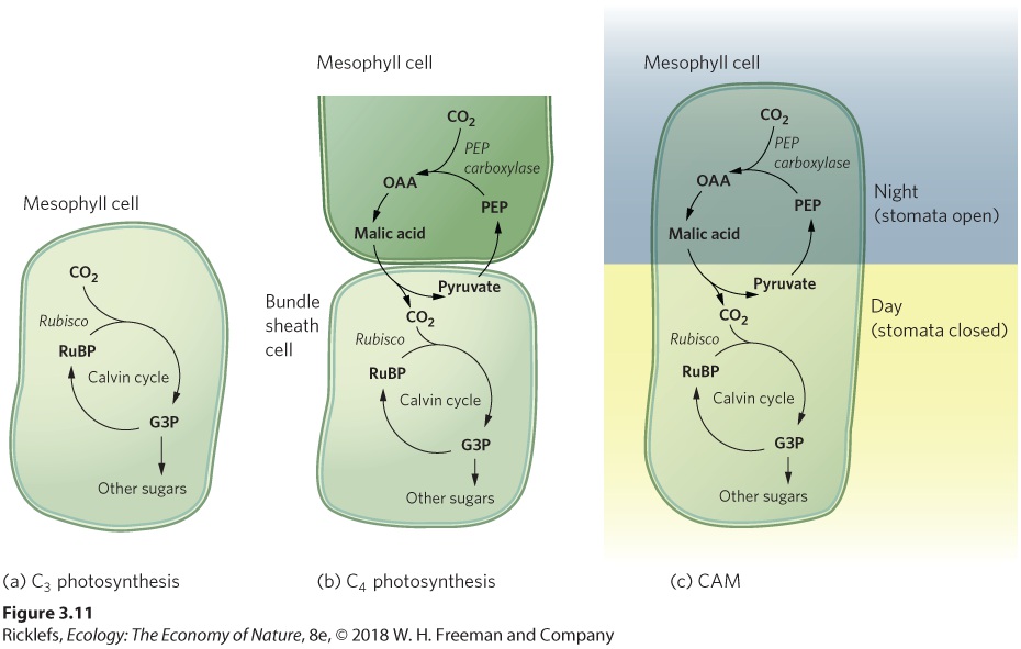
- Photosynthesis
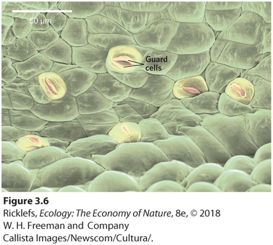
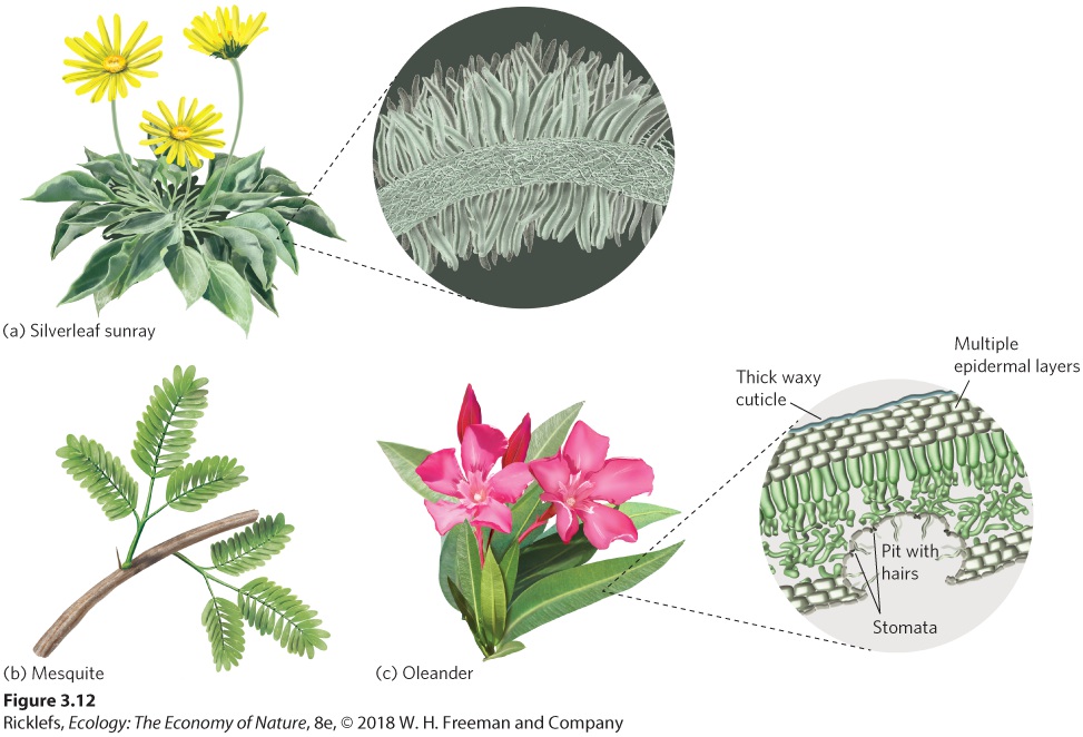
- Structural Adaptations to Water Stress
- Water and Salt Balance in Animals
- Water and Nitrogen Balance in Animals
- Analyzing Ecology

Ch 4Adaptations to Variable EnvironmentsRead full chapter →
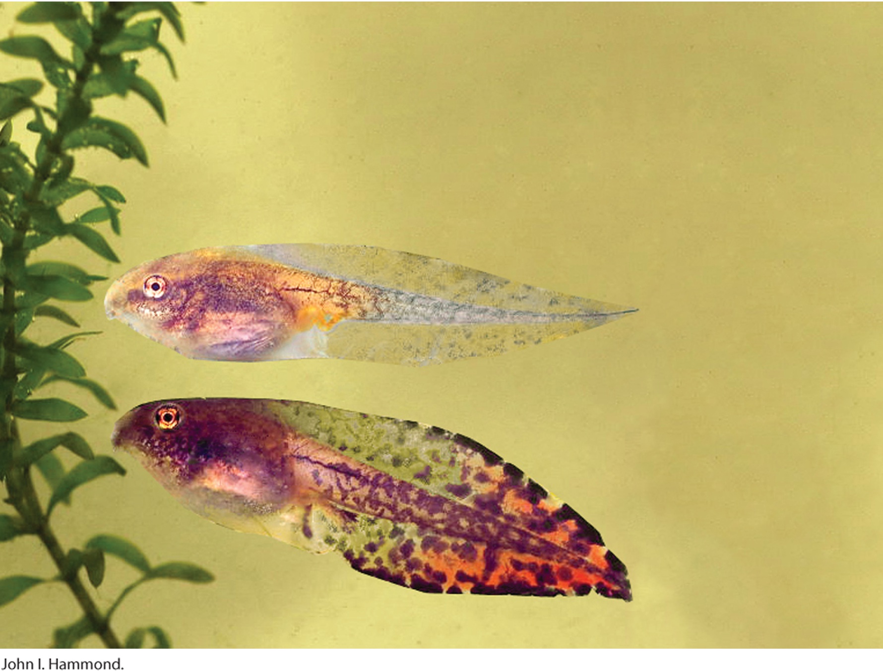
4Adaptations to Variable Environments Gray treefrog tadpoles. Tadpoles of the gray treefrog that live without predators exhibit high activity and develop relatively small tails that are drab. In contrast, tadpoles raised with predators exhibit low activity and develop large, red tails. The Fine-Tuned Phenotypes of Frogs Every spring the female gray treefrog (Hyla versicolor) must choose where she will lay her eggs. The treefrog is a medium-sized frog that lives throughout much of eastern North America and through the central United States to the Gulf Coast of Texas. As adults, they spend most …
Sections in this chapter
- 4 Adaptations to Variable Environments
- Learning Objectives
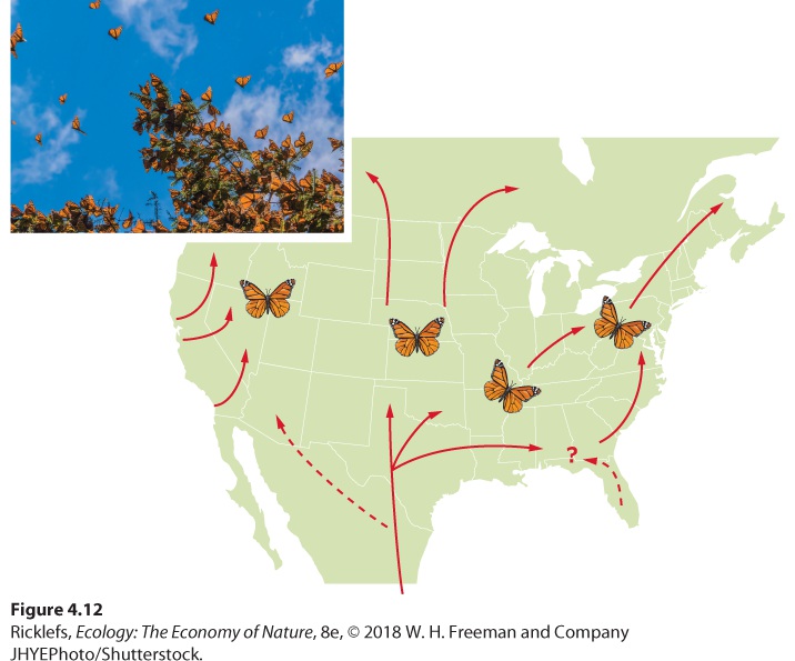
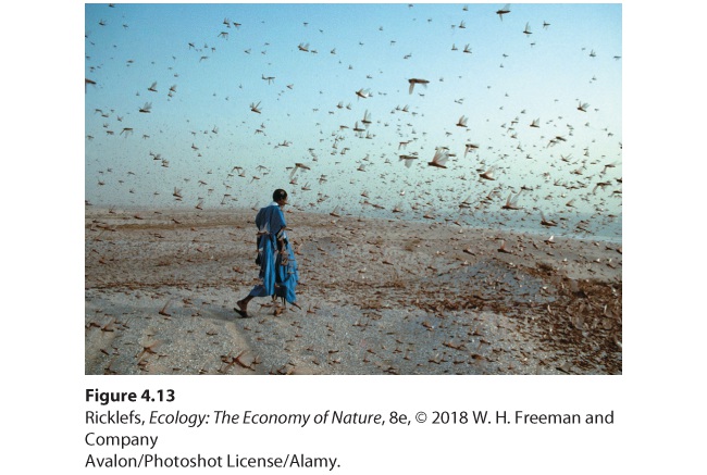
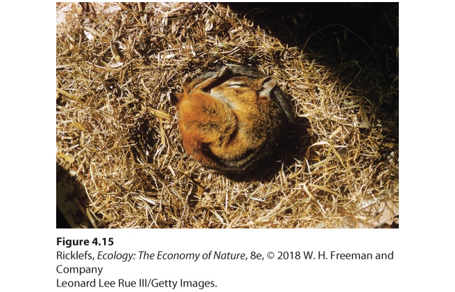
- Temporal Environmental Variation
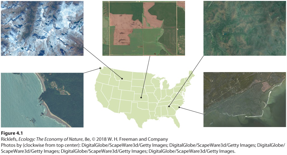
- Spatial Environmental Variation
- Phenotypic Trade-Offs
- Environmental Cues
- Response Speed and Reversibility
- Concept Check
- Competition for Scarce Resources
- Temperature
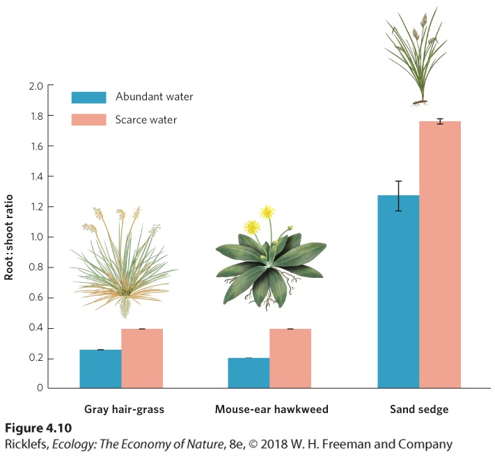
- Water Availability
- Salinity

Ch 5Climates and SoilsRead full chapter →
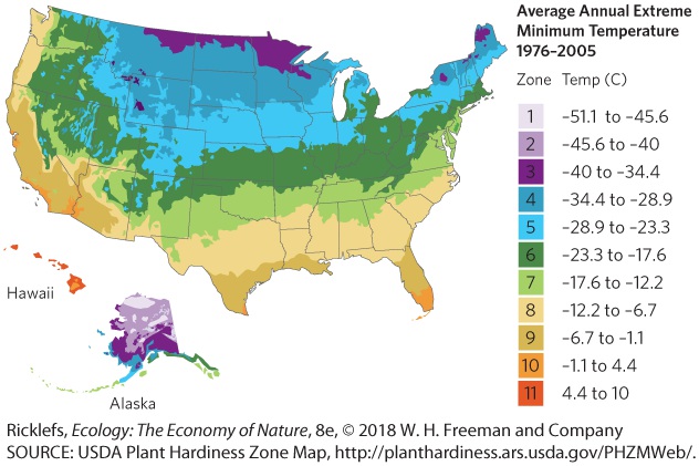
5Climates and Soils A beautiful garden. This garden is located at the Sequim Gardens, in Washington State. Where Does Your Garden Grow? If you have ever planted a garden, you know that you have a lot of decisions to make. You can choose from a vast selection of fruits and vegetables, not to mention a dizzying array of flowers, shrubs, and trees. Although you have a large number of choices, not all plants grow well in all locations. To help gardeners determine what plants can survive and flourish in their location, the U.S. Department of Agriculture has developed a map of plant hardiness zones.…
carry cold air from the middle of the continent toward the coast and push the warm ocean air away from the coast. As a result, the East Coast remains colder than the West Coast during the winter. The map of plant hardiness zones illustrates how climates around the world are the result of a complex combination of sunlight, latitude, elevation, air currents, and ocean currents. In this chapter, we will explore how global processes affect the distribution of climates on Earth and how climates affect the types of soils that form. Plant hardiness zones for North America. The warmest zones occur in …
Sections in this chapter
- 5 Climates and Soils
- Learning Objectives
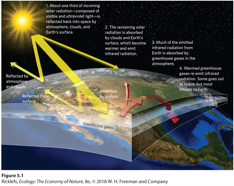
- The Greenhouse Effect
- Greenhouse Gases
- Concept Check
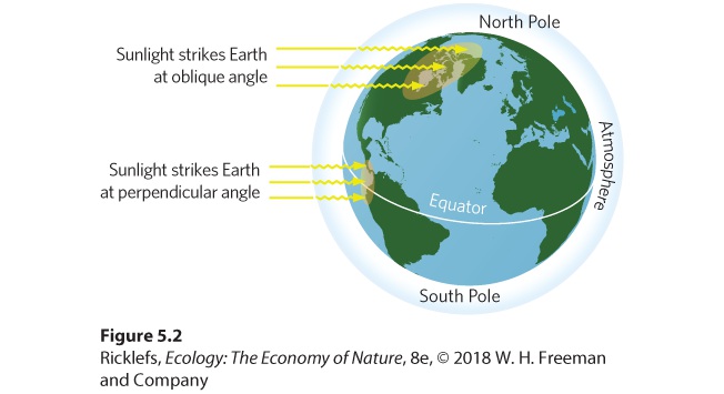
- The Path and Angle of the Sun
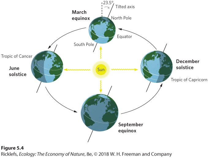
- Seasonal Heating of Earth
- Analyzing Ecology
- Properties of Air
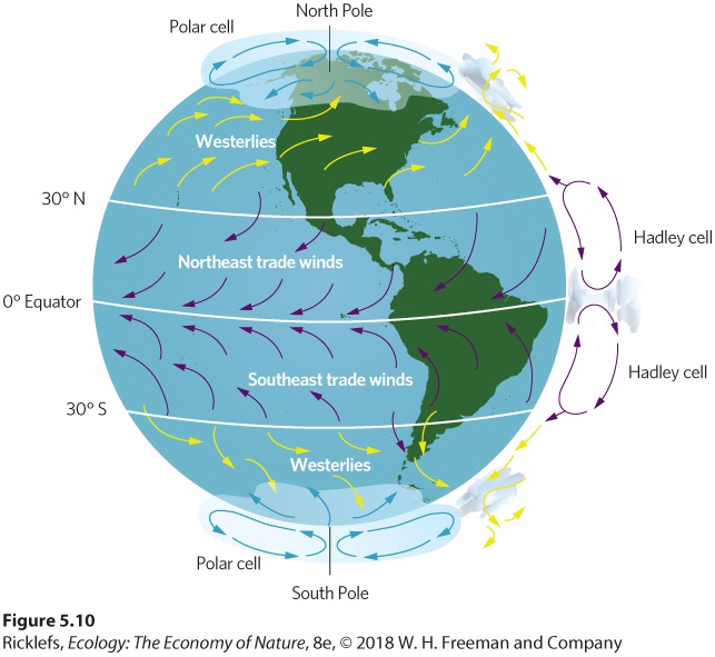
- Formation of Atmospheric Convection Currents
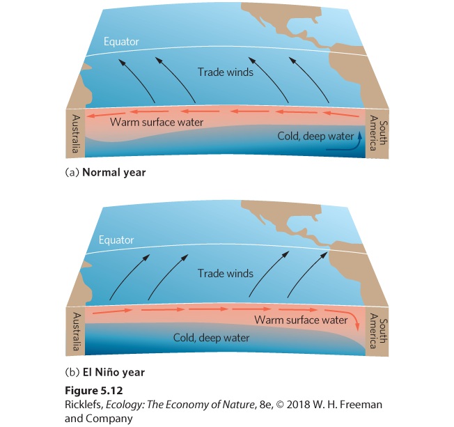
- Upwelling
- Thermohaline Circulation
Ch 6Terrestrial and Aquatic BiomesRead full chapter →
6Terrestrial and Aquatic Biomes Growing grapes for wine during the hot, dry summer. At the Chateau Corcelles in southern France, the climate is ideal for growing the grapes that are used for wine. The World of Wine The fascinating history of winemaking dates back thousands of years. Archaeologists have found signs of winemaking in many cultures around the Mediterranean Sea, including those of the ancient Egyptians, Romans, and Greeks. Indeed, the entire Mediterranean region has a long tradition of cultivating wine grapes, and the production of wine has played an important role in the economic …
plants, despite being separated by thousands of kilometers. For example, while each winemaking region contains a large number of unique plant species, the plants are similar in their growth form. Whether in France, California, Chile, or South Africa, the plant communities are dominated by drought-adapted grasses, wildflowers, and shrubs. In this chapter, we will explore how particular climates that are found in different locations around the world are associated with very similar-looking plants and how scientists use these patterns to categorize terrestrial ecosystems. We will also examine why…
Sections in this chapter
- 6 Terrestrial and Aquatic Biomes
- Learning Objectives
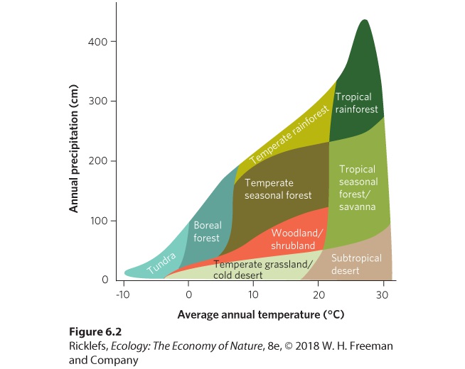
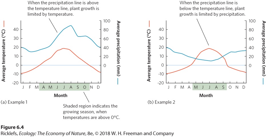
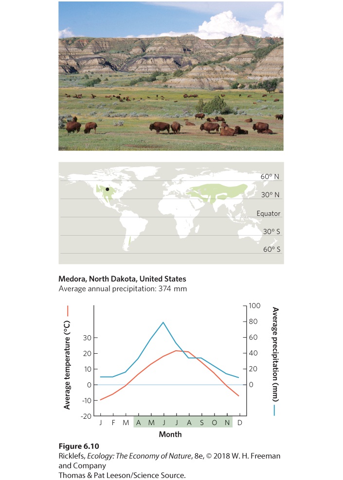
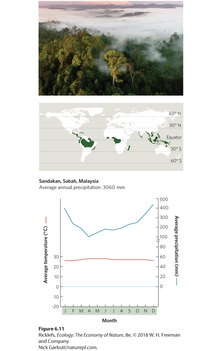
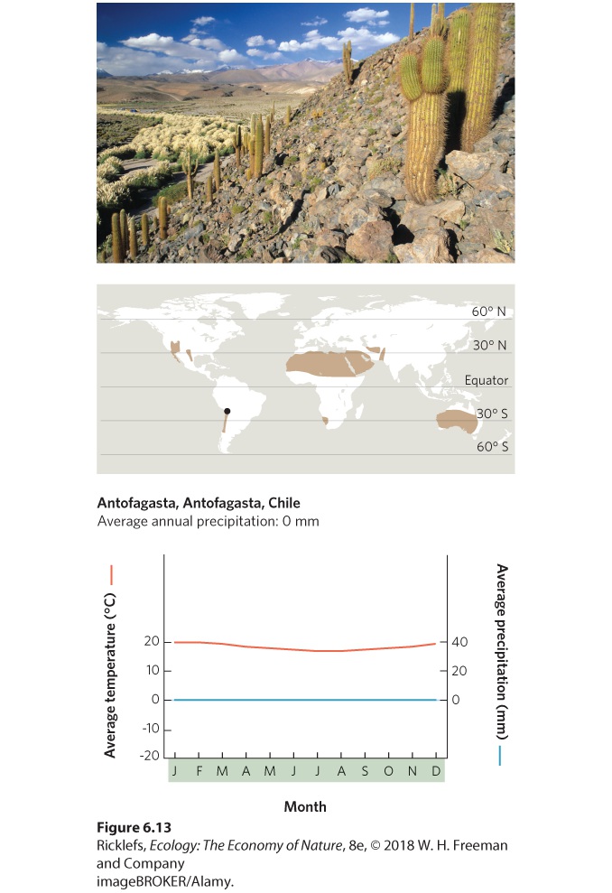
- Climate Diagrams
- Analyzing Ecology
- Concept Check
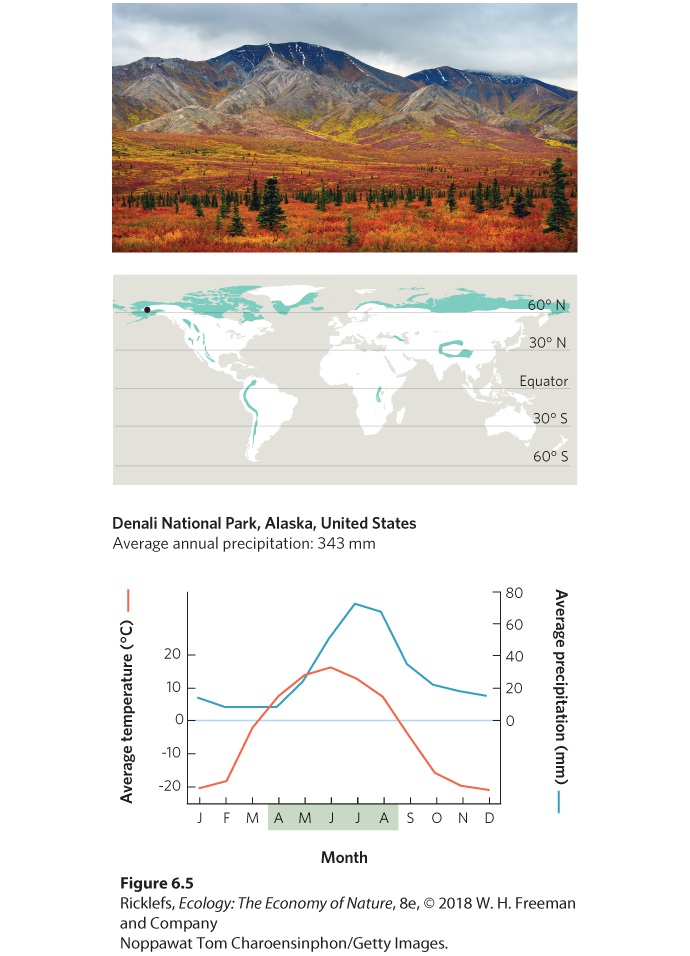
- Boreal Forests
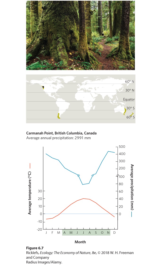
- Temperate Rainforests
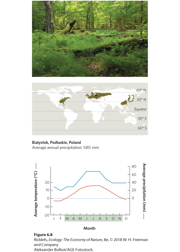
- Temperate Seasonal Forests
- Woodlands/Shrublands
- Temperate Grasslands/Cold Deserts
- Tropical Rainforests
- Tropical Seasonal Forests/Savannas
Ch 7Evolution and AdaptationRead full chapter →
7Evolution and Adaptation Ratite birds. Two-wattled Cassowary (Casuarius casuarius) female on a forest edge in Australia, Queensland, Moresby Range National Park. Favoring Flightless Birds One of the distinguishing characteristics of birds is that they possess feathers that help them fly. However, not all birds have the ability to fly, including penguins and a group of birds known as ratites. Ratites are a group of well-known species, such as the ostriches of Africa (Struthio spp.), the emus and cassowaries of Australia (Dromaius spp., Casuarius spp.), the kiwis of New Zealand (Apteryx spp.), …
The evolution of reduced flight muscles on predator-free islands also means that these birds are more susceptible to any predators that are introduced to the islands. As we will see in later chapters, the unintentional introduction of non-native bird predators, such as snakes, has decimated the bird fauna of many islands. The research on bird flight is just one example of how scientists can use the theory of evolution by natural selection to obtain tremendous insight into how natural selection operates in nature. By studying how evolution occurs in wild populations, we can see how natural sele…
Sections in this chapter
- 7 Evolution and Adaptation
- Learning Objectives
- The Structure of Dna
- Genes and Alleles
- Dominant and Recessive Alleles
- Sources of Genetic Variation
- Concept Check
- Evolution Through Random Processes
- Evolution Through Selection, A Nonrandom Process
- Analyzing Ecology
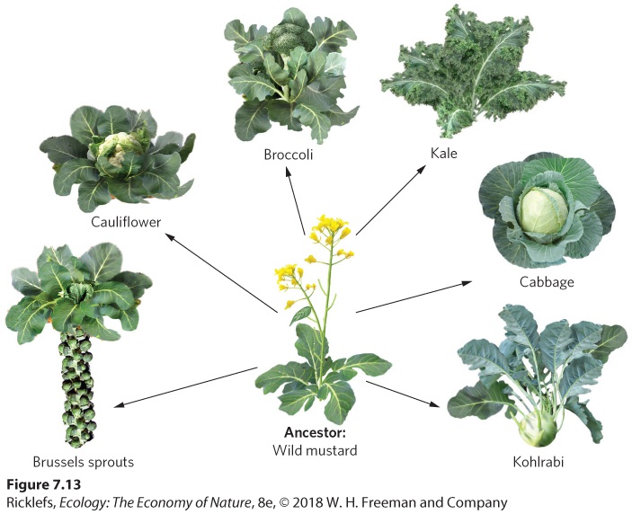
- Artificial Selection
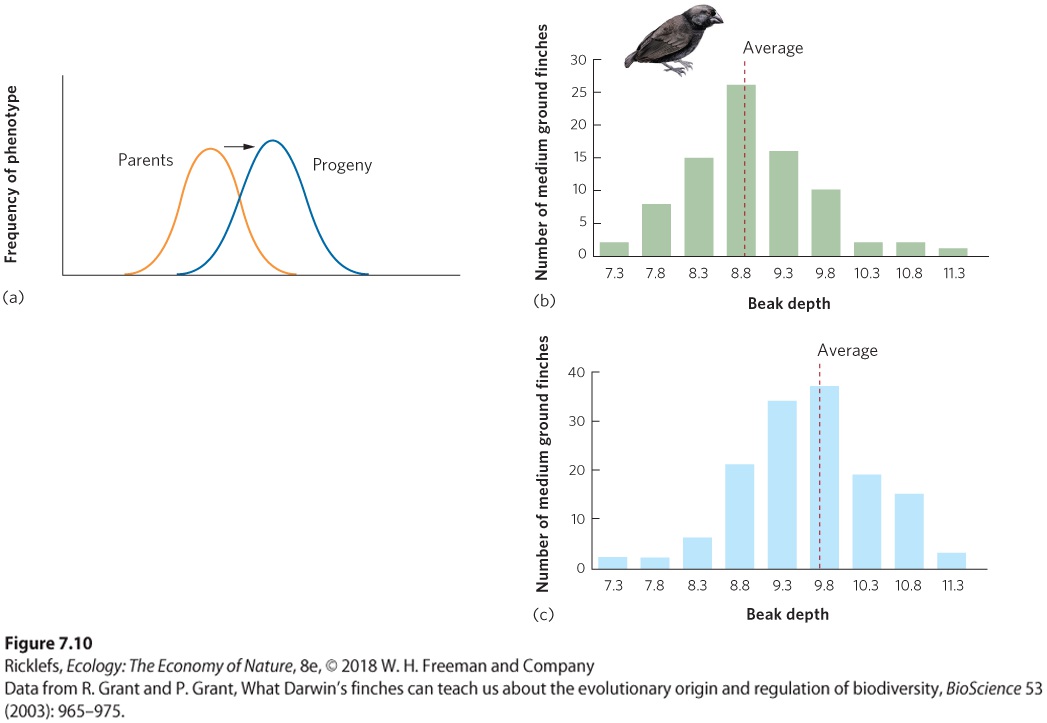
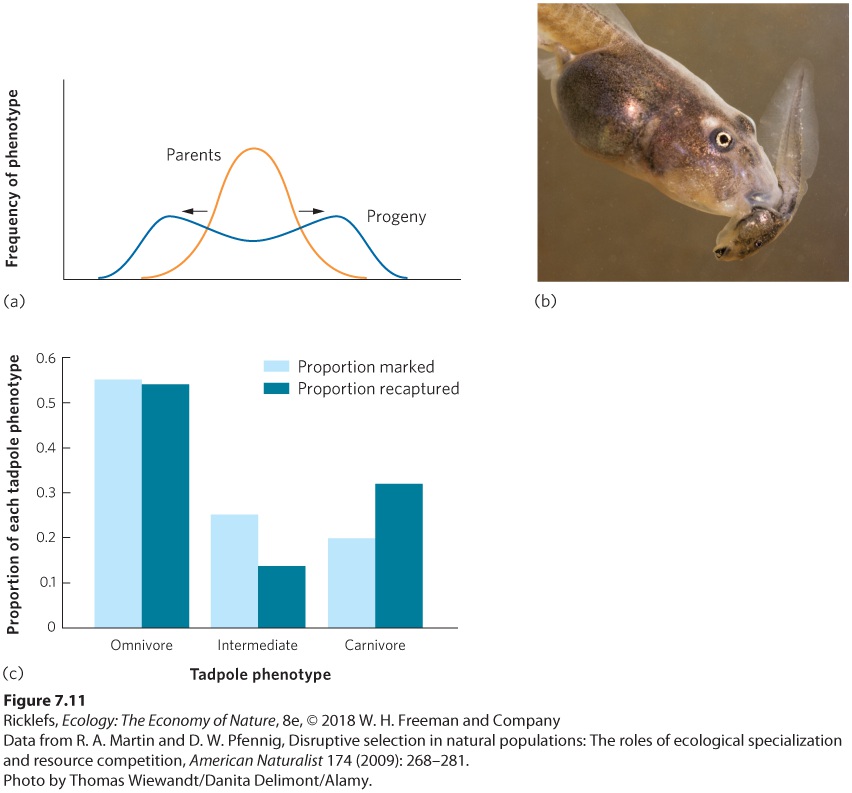
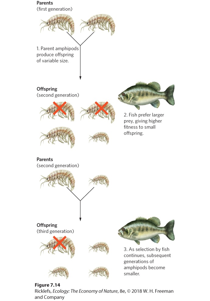
- Natural Selection
Ch 8Life HistoriesRead full chapter →
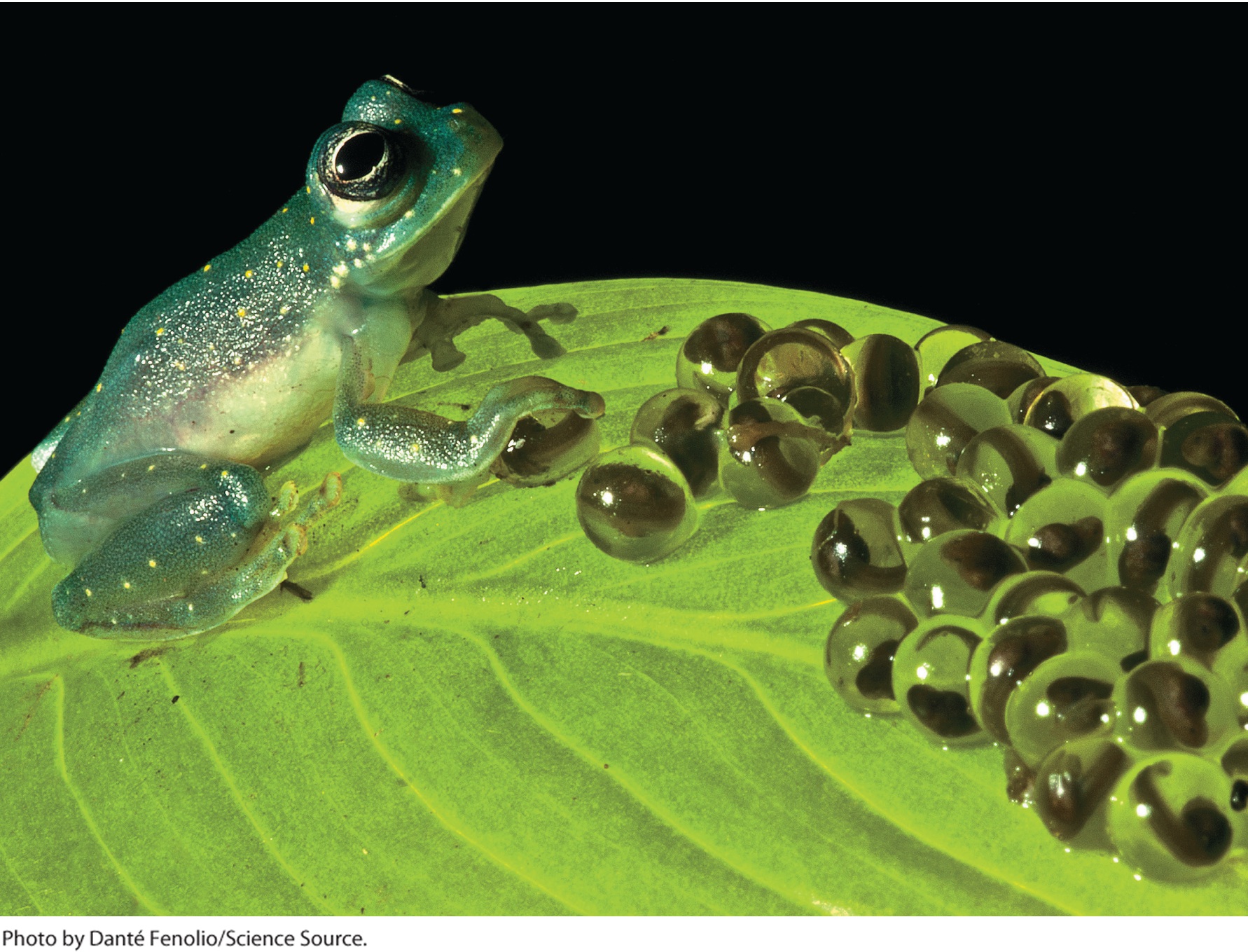
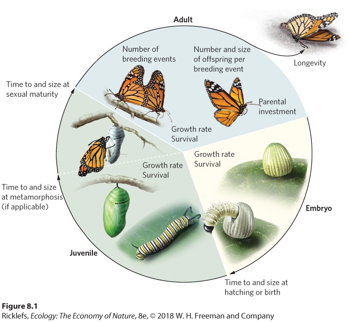
8Life Histories Reproduction in frogs. While many frogs have a typical life of hatching into a tadpole that later metamorphoses into a frog, other species skip the entire tadpole stage by hatching into a tiny froglet. The Many Ways to Make a Frog When we think of a frog’s life, we often think of an egg hatching into a tadpole, the tadpole growing larger, and ultimately metamorphosing into a frog. Within this lifestyle, there is tremendous variation; some species of frogs spend up to 2 years as a tadpole, whereas other species spend as few as 10 days. In addition, the number of eggs laid can ra…
energy in the form of yolk. The diversity of frog reproduction highlights the notion that species on Earth have evolved a tremendous variety of reproductive strategies. As we shall see in this chapter, organisms have evolved a wide range of alternative strategies for growth, development, and reproduction, and these commonly reflect important fitness trade-offs. SOURCES: Gomez-Mestre, et al. 2012. Phylogenetic analyses reveal unexpected patterns in the evolution of reproductive modes in frogs. Evolution 66: 3687–3700.
Sections in this chapter
- 8 Life Histories
- Learning Objectives
- The Slow-To-Fast Life History Continuum
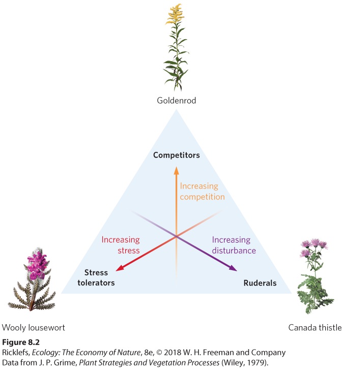
- Combinations of Life History Traits in Plants
- Concept Check
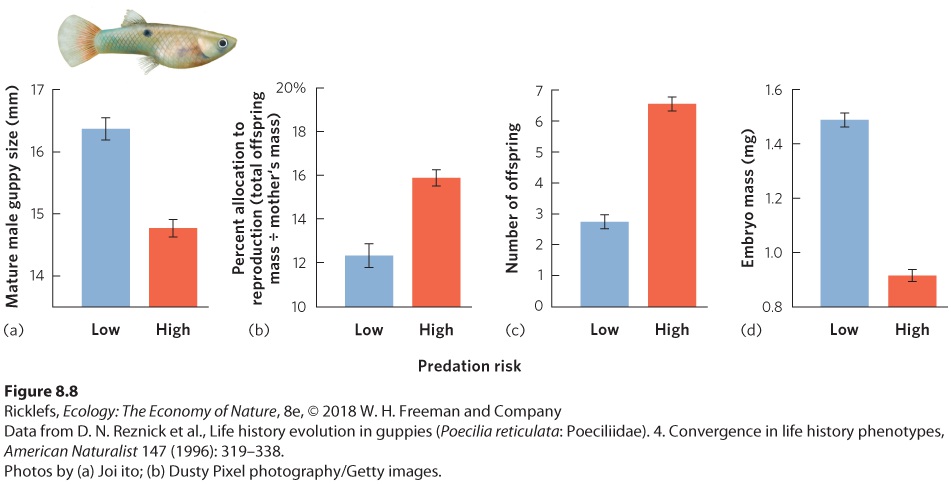
- The Principle of Allocation
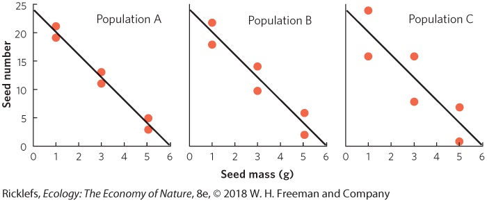
- Offspring Number Versus Offspring Size
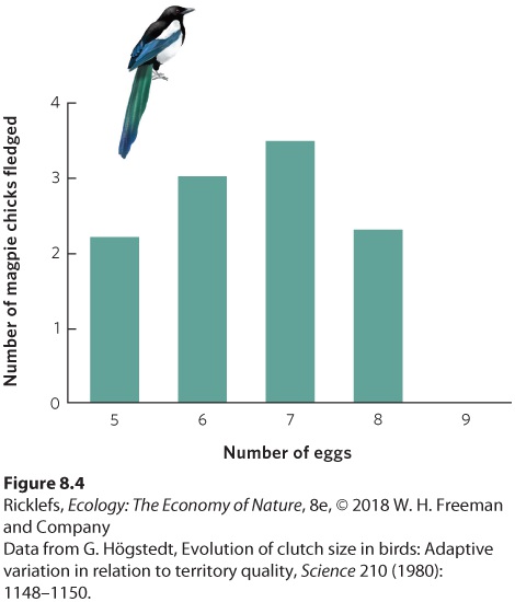
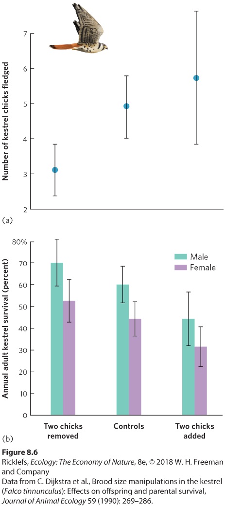
- Offspring Number Versus Parental Care
- Analyzing Ecology
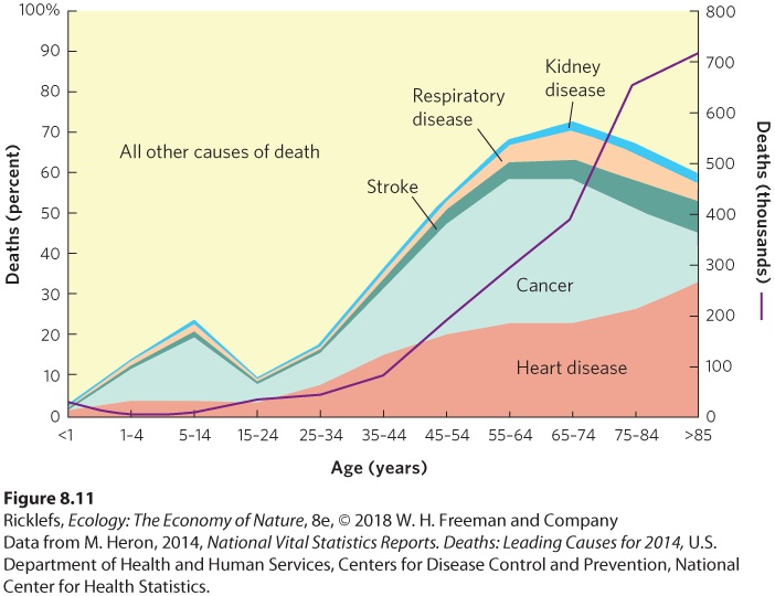
- Survival
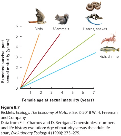
- Growth Versus Age of Sexual Maturity and Life Span
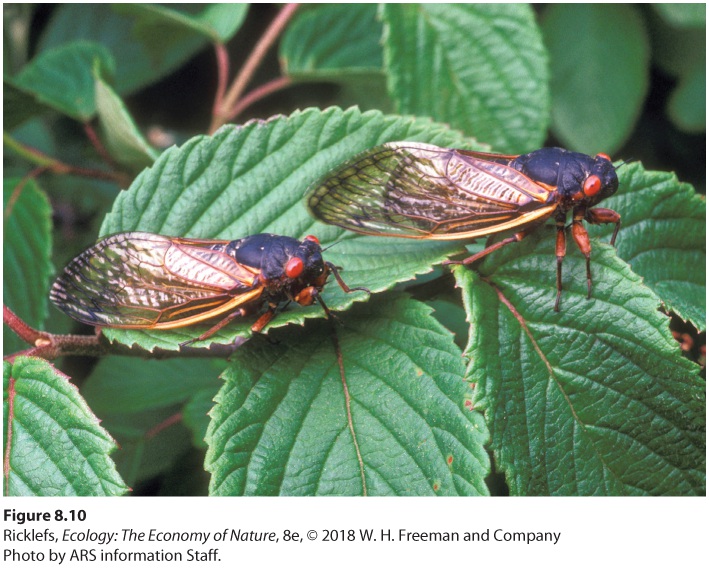
- Semelparity and Iteroparity
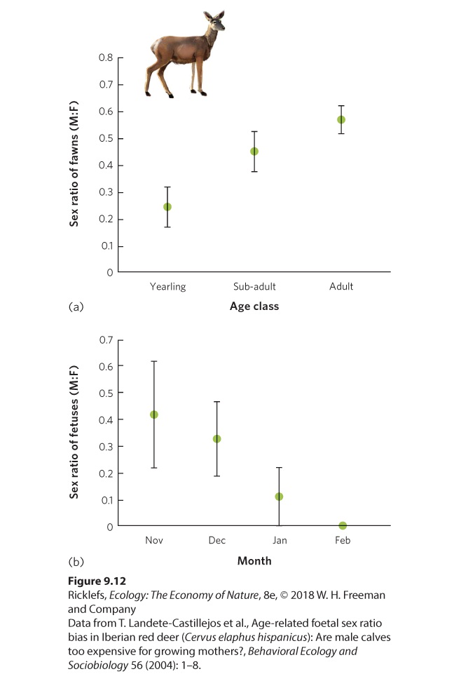
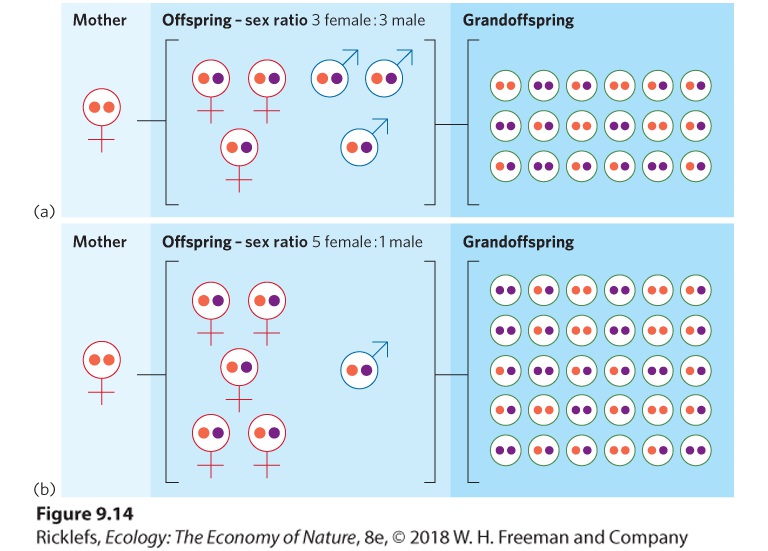
Ch 9Reproductive StrategiesRead full chapter →
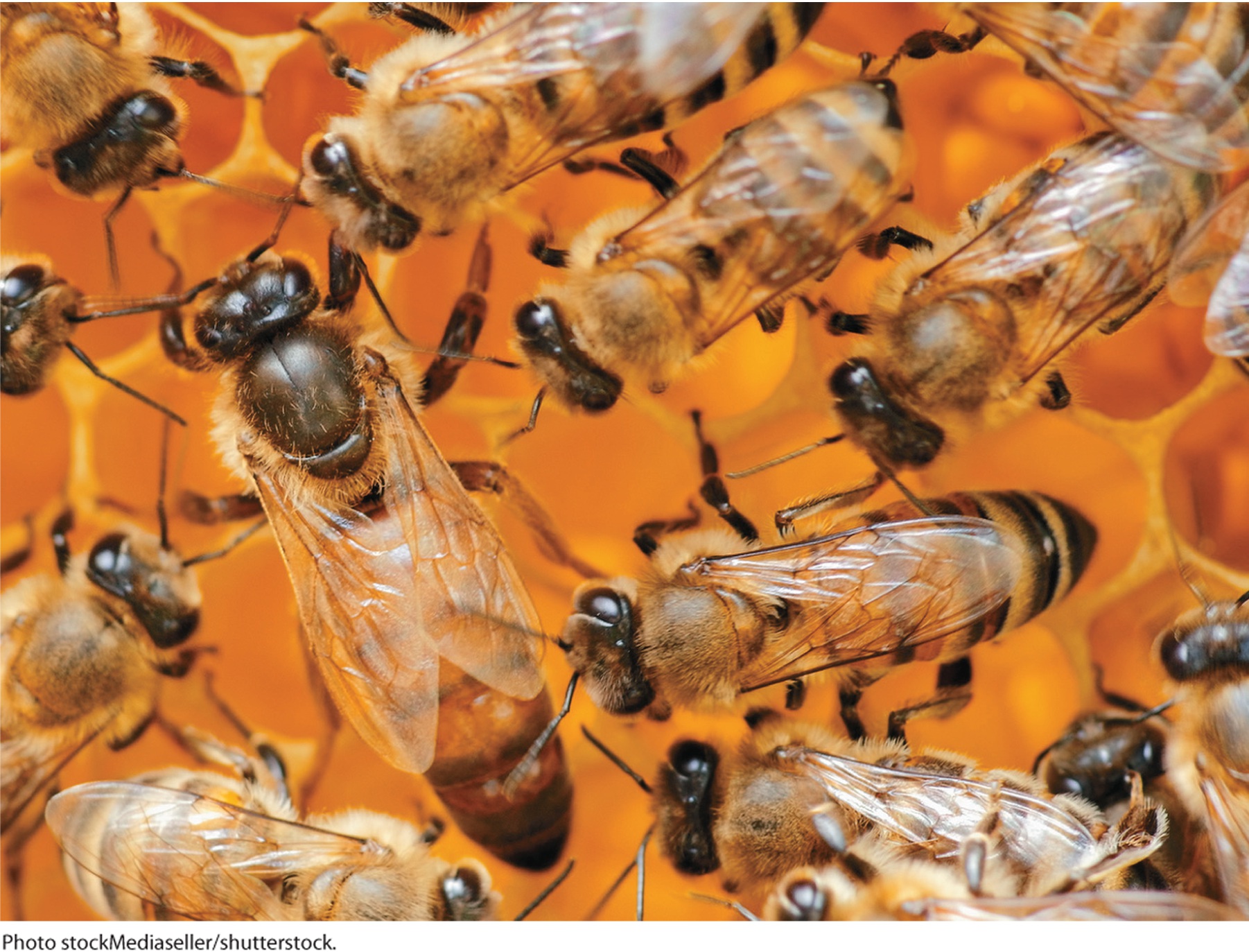
9Reproductive Strategies A honeybee hive. In most populations of honeybees, a queen can reproduce by laying either haploid eggs that produce sons or fertilized diploid eggs that produce daughters. The Sex Life of Honeybees Honeybees (Apis mellifera) have a complicated sex life. They live in hives that may contain tens of thousands of bees, usually progeny of the same mother, known as the queen. Like many organisms, the queen bee produces sons and daughters, but she does so in a rather unique way. Early in her life, the queen bee flies out of the hive and mates in the air with a group of male b…
Sections in this chapter
- 9 Reproductive Strategies
- Learning Objectives
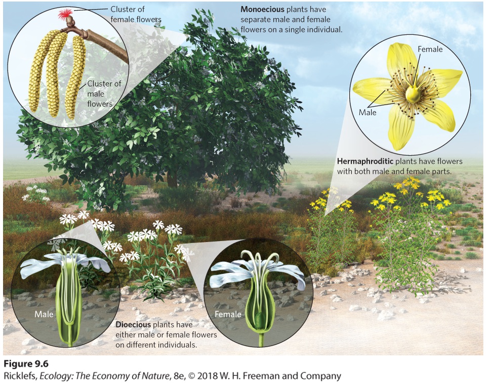
- Sexual Reproduction
- Asexual Reproduction
- Costs of Sexual Reproduction
- Benefits of Sexual Reproduction
- Concept Check
- Comparing Strategies
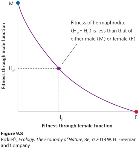
- Selfing Versus Outcrossing of Hermaphrodites
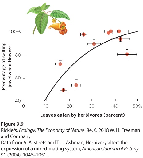
- Mixed Mating Strategies
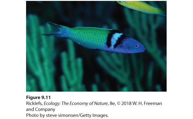
- Mechanisms of Sex Determination
- Offspring Sex Ratio
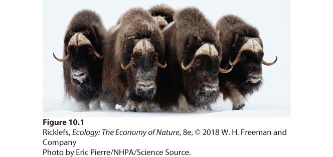
Ch 10Social BehaviorsRead full chapter →
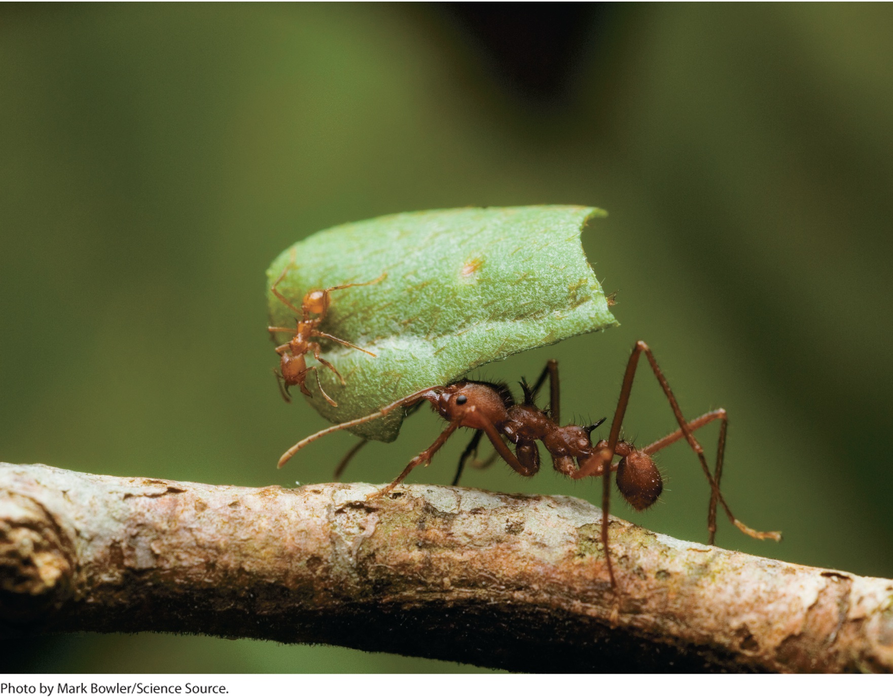
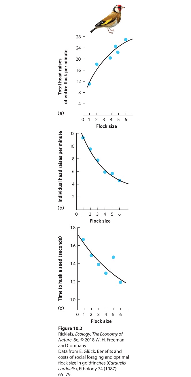
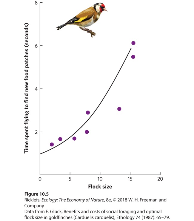
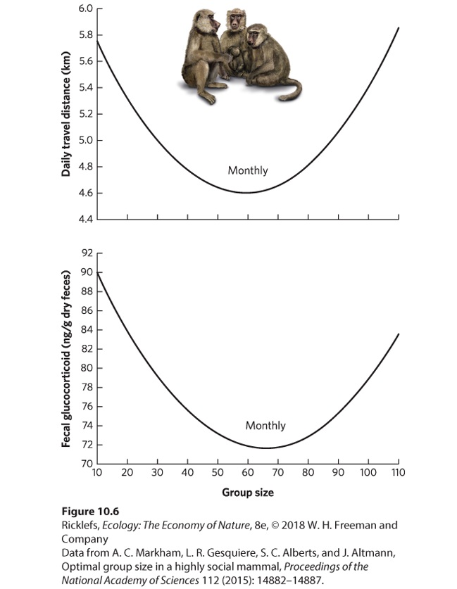
10Social Behaviors Leaf-cutter ants. Through an extensive division of labor, leaf-cutter ants work together to bring pieces of leaves back to their nest. In this photo, a large worker ant carries a cut piece of leaf, while a much smaller worker ant rides on top to discourage parasitoid flies from attacking the worker. The Life of a Fungus Farmer The leaf-cutter ant is an extraordinary farmer. Living in colonies of several million individuals, these ants leave the colony each day to harvest leaves from the surrounding forest. Using their sharp mandibles, they slice through leaves to cut off pie…
Sections in this chapter
- 10 Social Behaviors
- Learning Objectives
- Benefits of Living in Groups
- Costs of Living in Groups
- Territories
- Dominance Hierarchies
- Concept Check
- The Types of Social Interactions
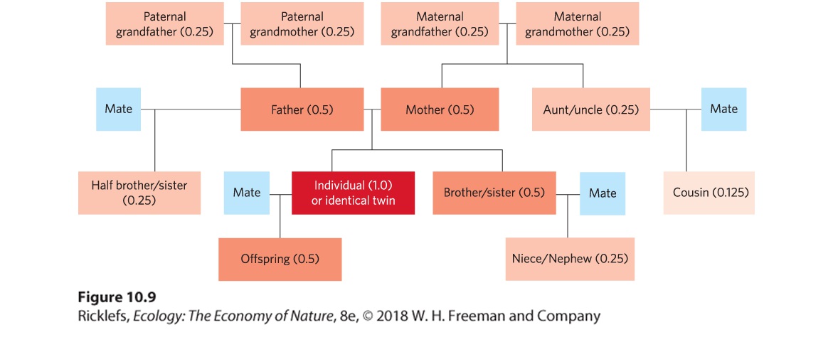
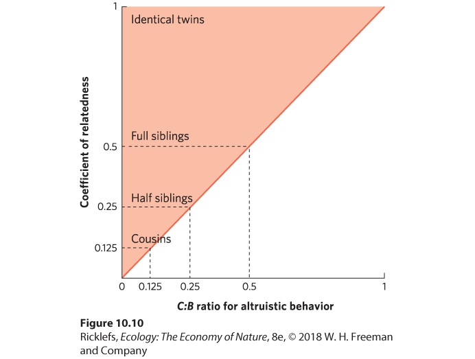
- Altruism and Kin Selection
- Analyzing Ecology
- Primary Helper
- Secondary
Ch 11Population DistributionsRead full chapter →
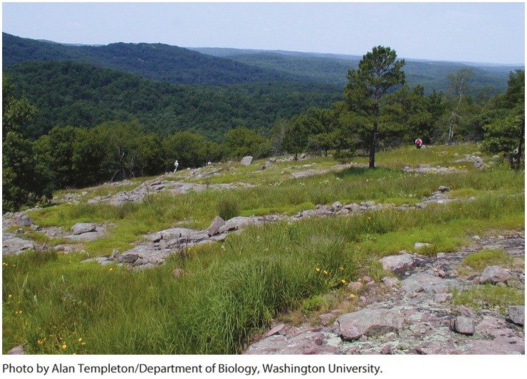
11Population Distributions A male collared lizard. Males of this species have a bright orange throat that intimidates other males and attracts females. Bringing Back the Mountain Boomer When Alan Templeton was a Boy Scout in 1960, he encountered his first collared lizards (Crotaphytus collaris), also known as mountain boomers, in the Ozark Mountains of Missouri. He was struck by the brightly colored males that ran around in the forest openings that dotted the mountains. Two decades later, as a biology professor at Washington University in St. Louis, he returned to the Ozark Mountains and was s…
Sections in this chapter
- 11 Population Distributions
- Learning Objectives
- Determining Suitable Habitats
- Ecological Niche Modeling
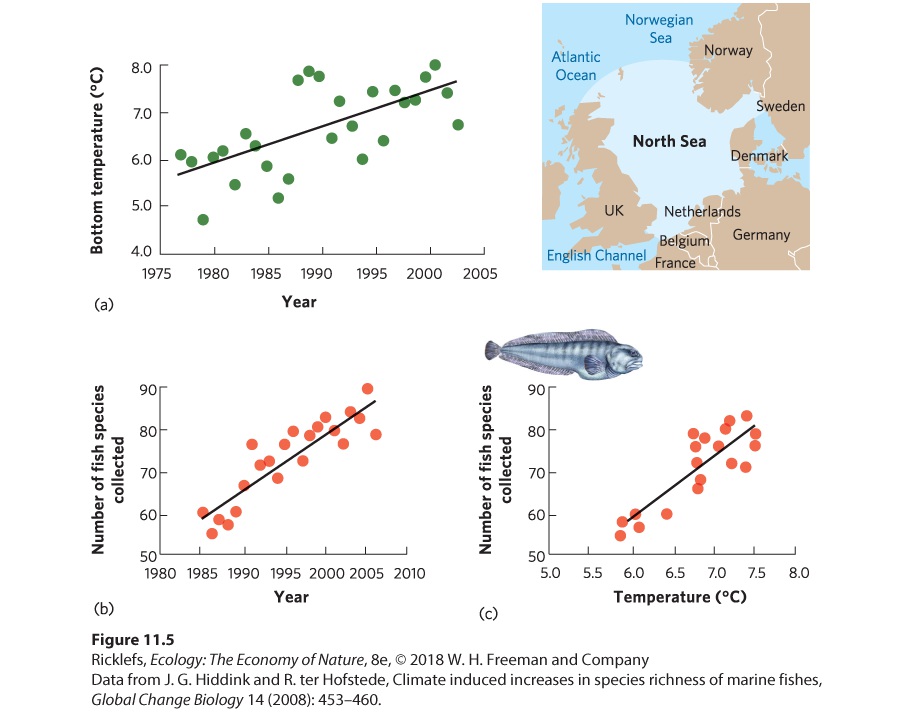
- Habitat Suitability and Global Warming
- Concept Check
- Geographic Range
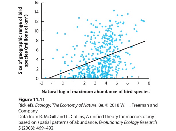
- Abundance
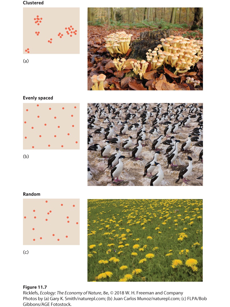
- Dispersion
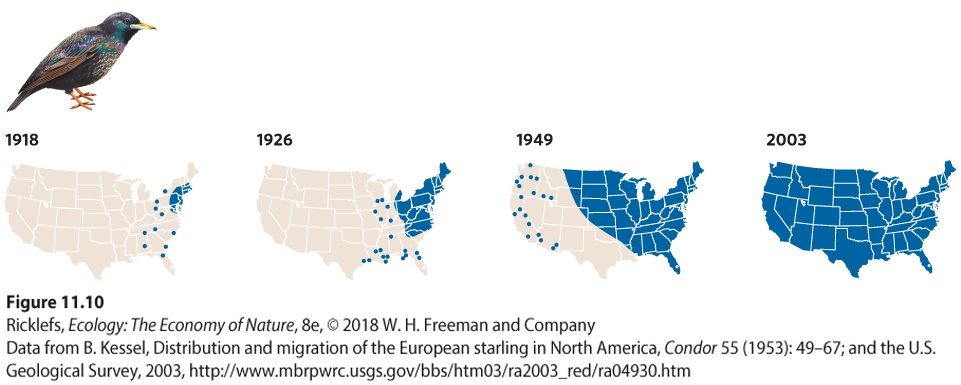
- Dispersal
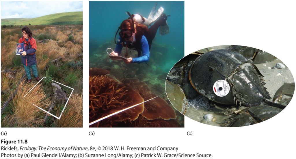
- Quantifying the Location and Number of Individuals
- Analyzing Ecology
Ch 12Population Growth and RegulationRead full chapter →
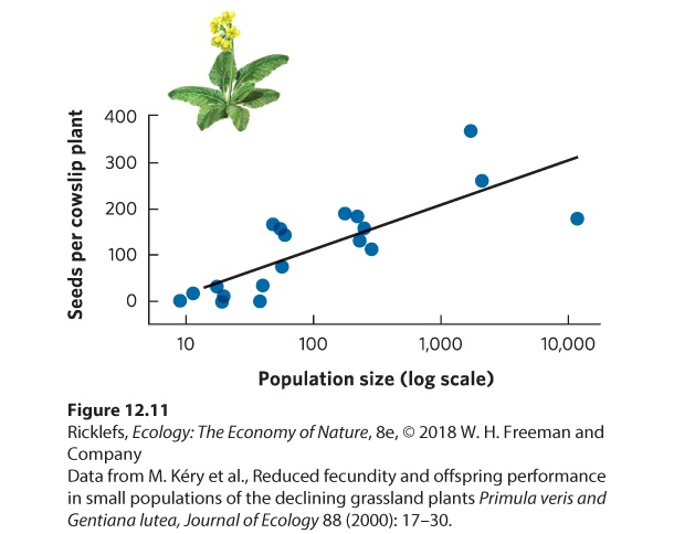
12Population Growth and Regulation Animal overpopulation. With the decline of top predators and an increase in suitable habitats, many large herbivores have dramatically increased in abundance to the point that it negatively affects native plants, other wildlife, and humans. In this photo, an overabundance of kangaroos graze on a golf course in Australia. Putting Nature on Birth Control We often hear about the decline of species around the world due to human activities, but some species are doing extraordinarily well. In particular, the populations of many large herbivores have increased to un…
Sections in this chapter
- 12 Population Growth and Regulation
- Learning Objectives
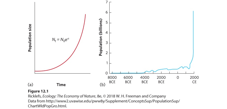
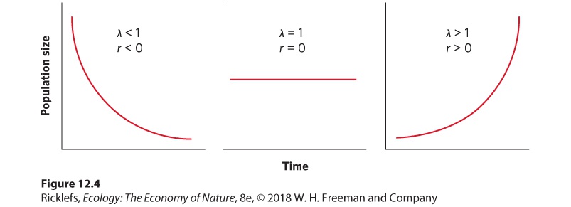
- The Exponential Growth Model
- The Geometric Growth Model
- Comparing the Exponential and Geometric Growth
- Population Doubling Time
- Concept Check
- Density-Independent Factors
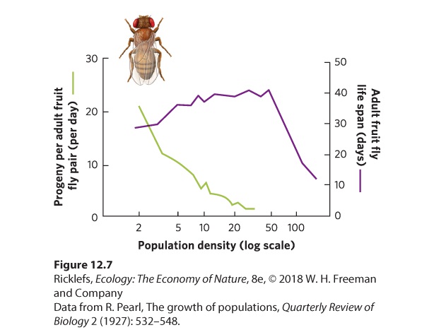
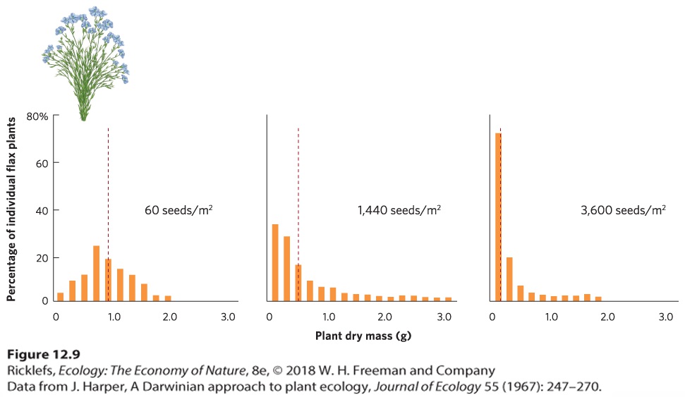
- Density-Dependent Factors
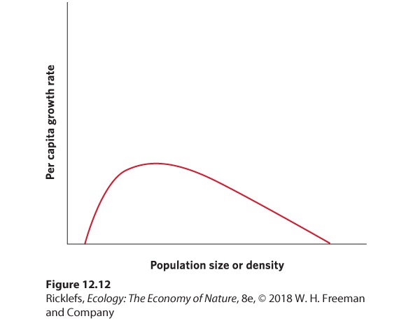
- Positive Density Dependence
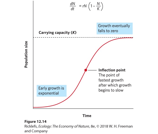
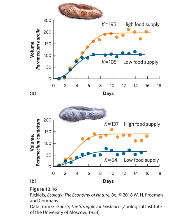
- The Logistic Growth Model
- Logistic Equation
Ch 13Population Dynamics over Space and TimeRead full chapter →
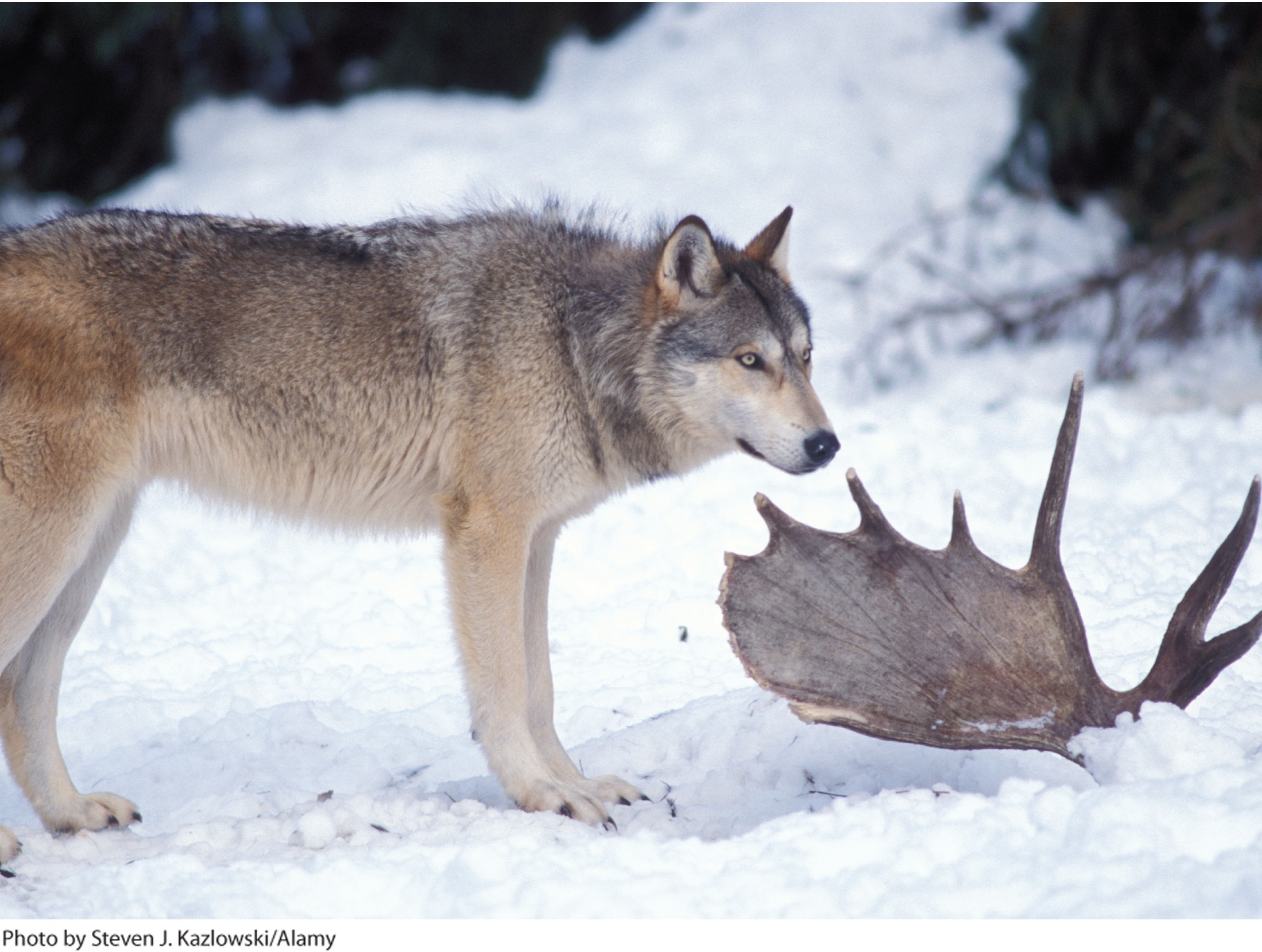
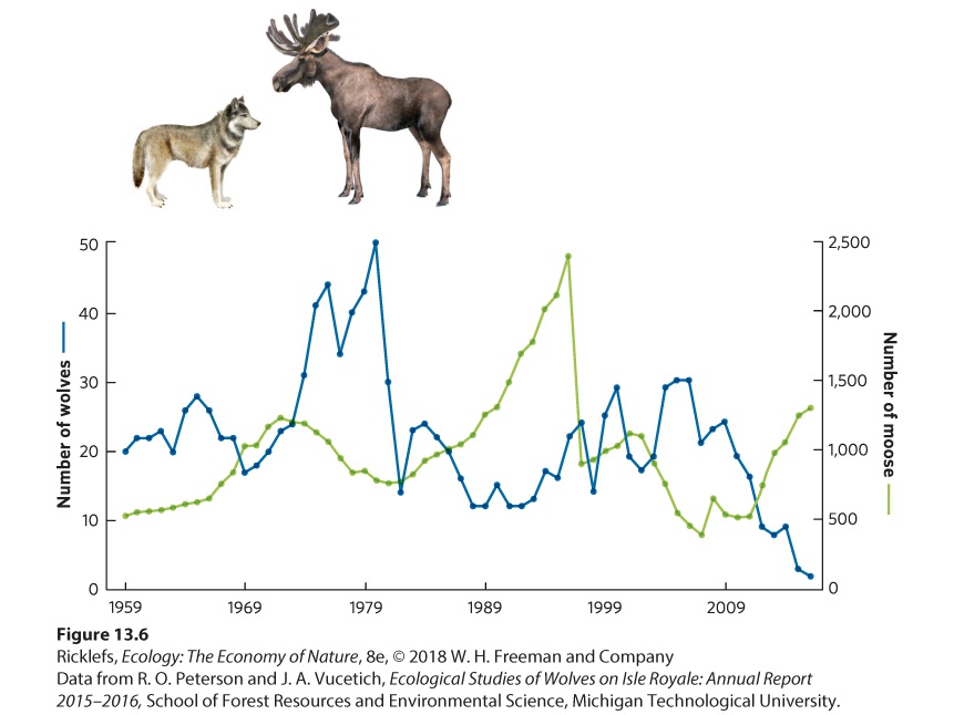
13Population Dynamics over Space and Time The wolves and moose of Isle Royale in Lake Superior. For more than 50 years, researchers have tracked large swings in moose and wolf population sizes. Monitoring Moose in Michigan Isle Royale, which is part of the state of Michigan and located off the northern shore of Lake Superior, has long served as a natural laboratory for ecologists. In the early 1900s, the island was colonized by moose from the mainland. This unlikely feat probably occurred during winter when the lake was frozen and the moose could travel the 40 km from the shores of the provinc…
Sections in this chapter
- 13 Population Dynamics over Space and Time
- Learning Objectives
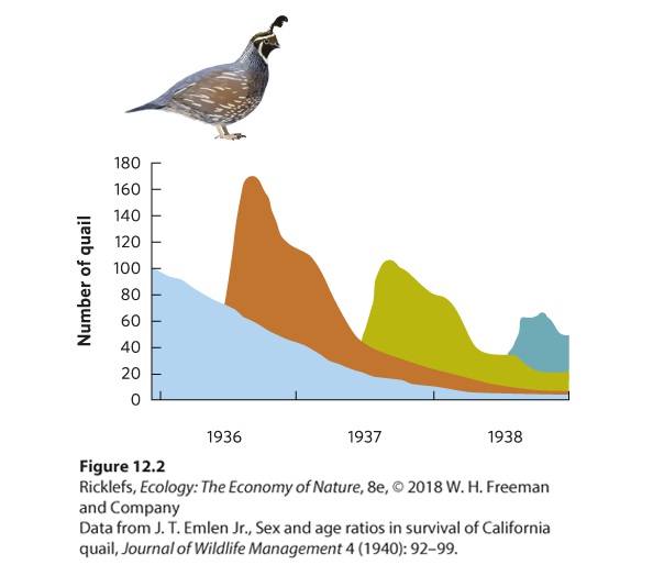
- Fluctuations in Age Structure
- Overshoots and Die-Offs
- Concept Check
- Capacities
- Delayed Density Dependence
- Population Sizes Cycle in Laboratory Populations
- Analyzing Ecology
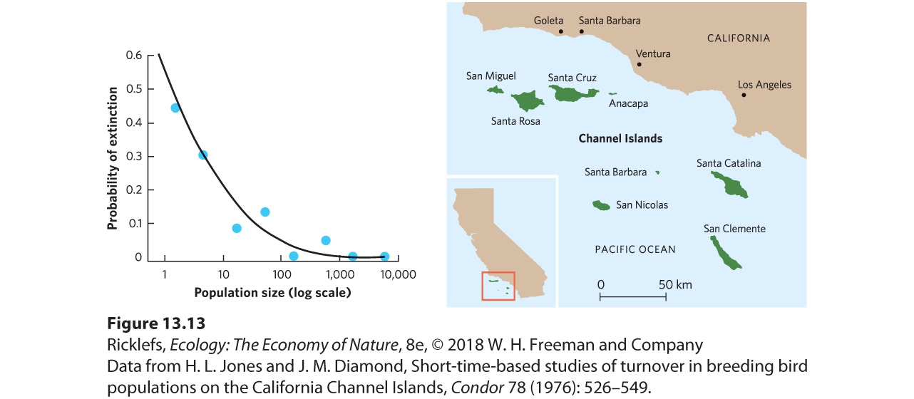
- Extinction in Small Populations
- Extinction Due to Variation in Population Growth
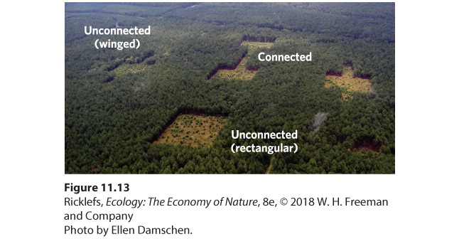
- The Fragmented Nature of Habitats
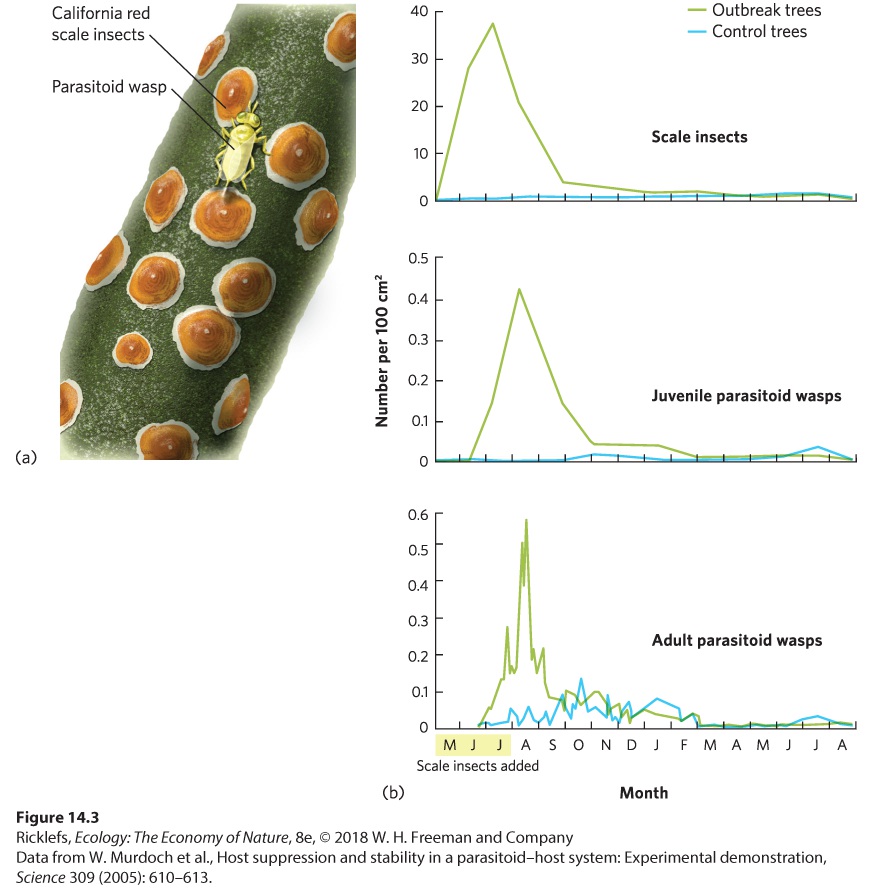
Ch 14Predation and HerbivoryRead full chapter →
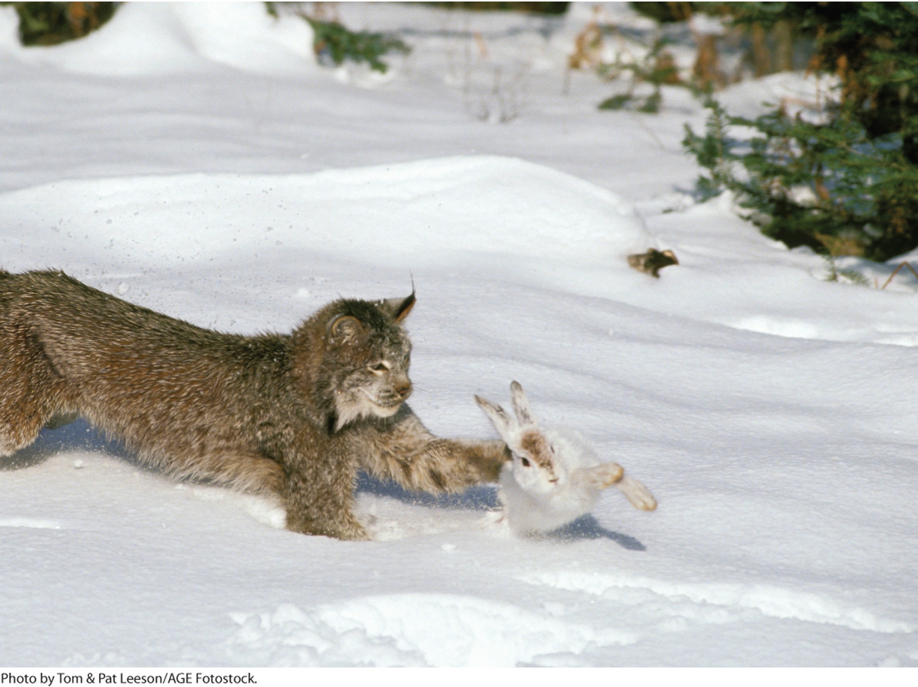
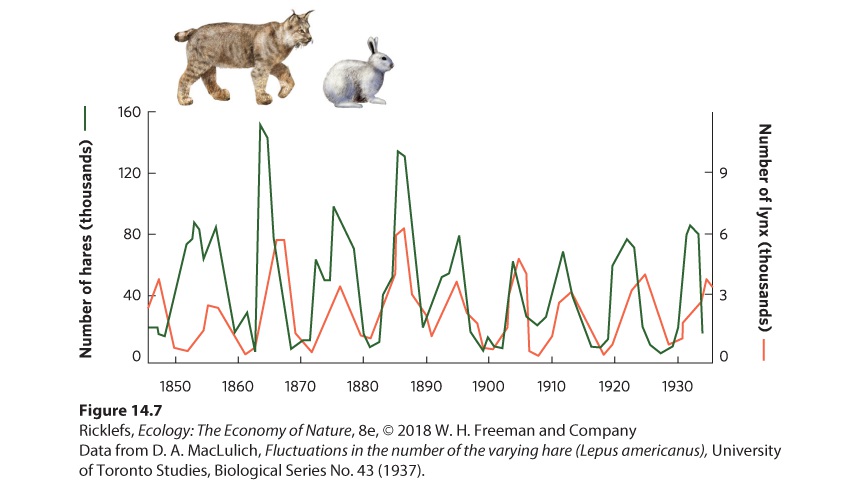
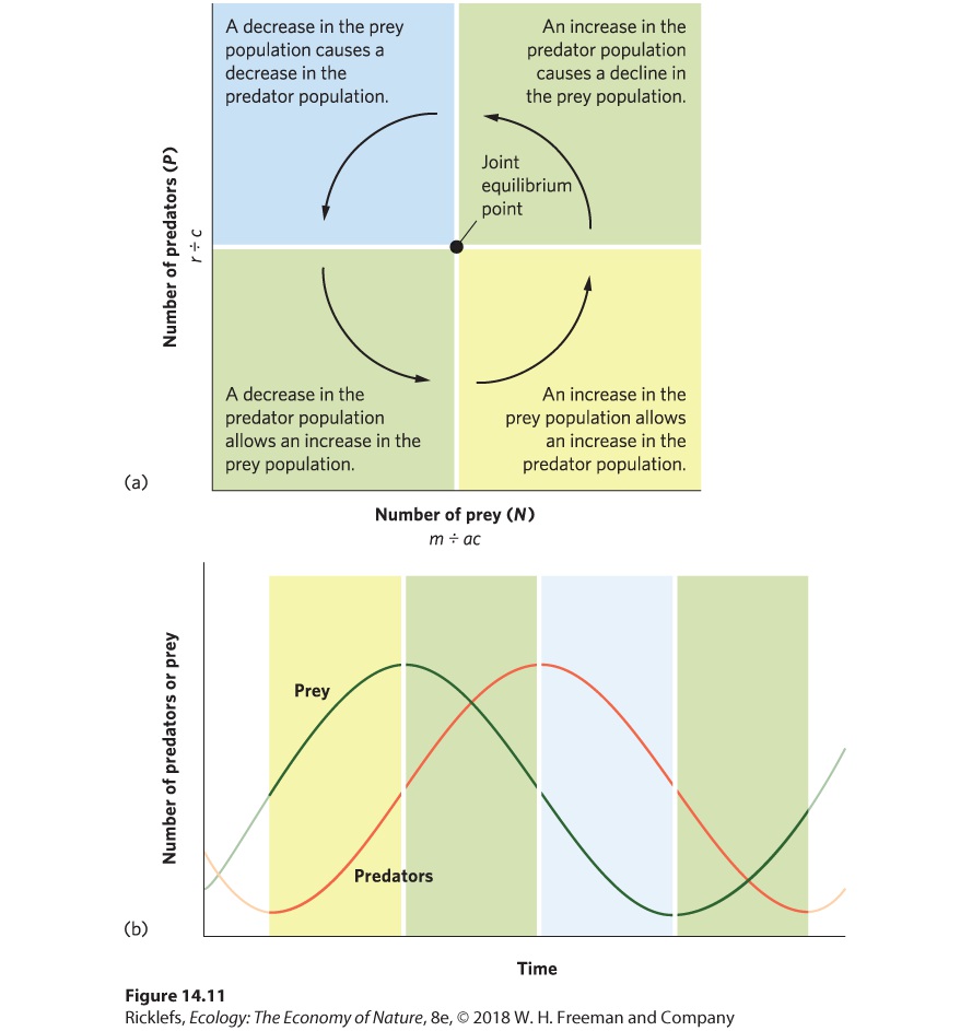
14Predation and Herbivory Canadian lynx and snowshoe hare. For nearly 100 years, ecologists have been examining the regular fluctuations in the populations of these species to determine the causes. A Century-Long Mystery of the Lynx and the Hare For centuries, naturalists, hunters, and trappers have noticed that populations of many species experience large fluctuations, and that some species fluctuate at regular intervals. In 1924, the ecologist Charles Elton drew attention to regular population fluctuations in many species of high-latitude animals in Canada, Scandinavia, and Siberia. In parti…
Sections in this chapter
- 14 Predation and Herbivory
- Learning Objectives
- Predators
- Mesopredators
- Herbivores
- Concept Check
- Functional and Numerical Responses
- Defenses Against Predators
- Analyzing Ecology
- Defenses Against Herbivores
- Concepts
- Summary of Learning Objectives
Ch 15Parasitism and Infectious DiseasesRead full chapter →
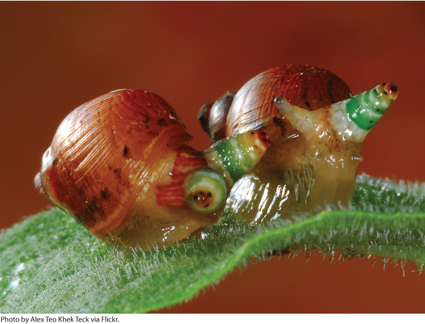
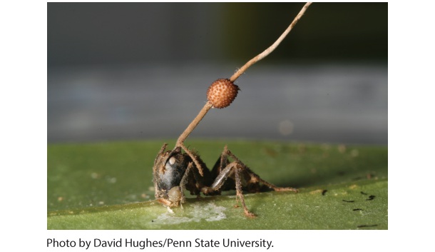
15Parasitism and Infectious Diseases A parasitized amber snail. The snail on the right has one normal eye stalk that is pale and slender and another that is infected by a parasitic flatworm, which causes the eye stalk to become enlarged and colorful. It also pulsates in a way that is attractive to predatory birds. The Life of Zombies Zombie films scare us because they depict zombies as the walking dead in search of victims they will turn into more zombies. But something similar to this happens commonly in nature; some species of parasites infect a host and take control of its life for their ow…
Sections in this chapter
- 15 Parasitism and Infectious Diseases
- Learning Objectives
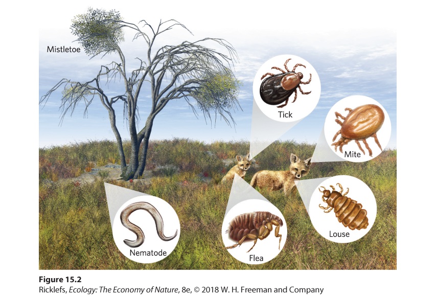
- Ectoparasites
- Endoparasites
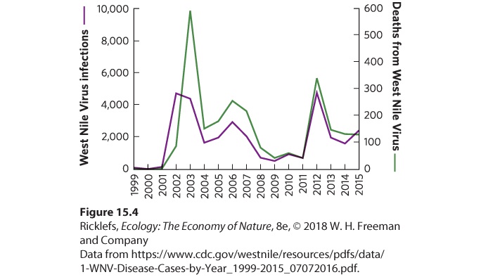
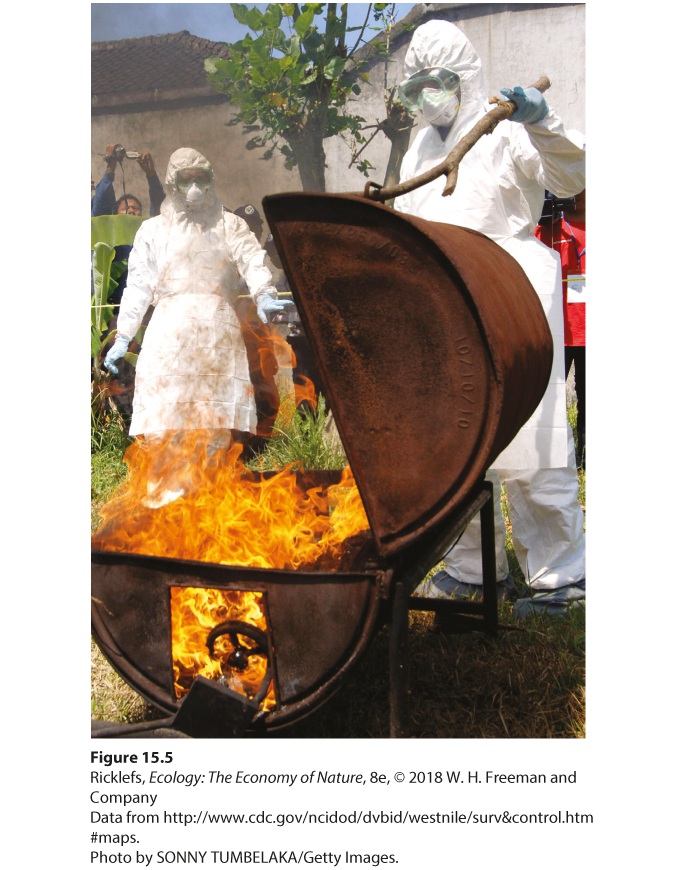
- Emerging Infectious Diseases
- Concept Check
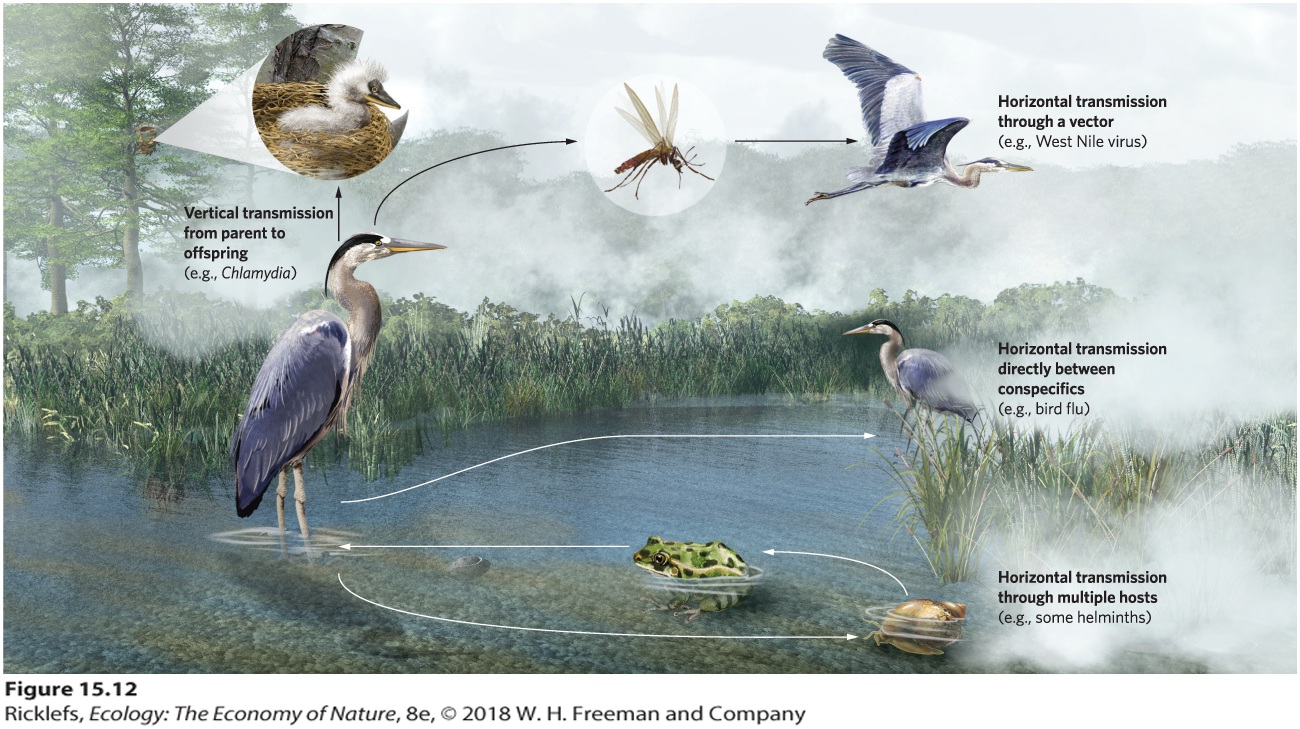
- Mechanisms of Parasite Transmission
- Modes of Entering the Host
- Jumping between Species
- Reservoir Species
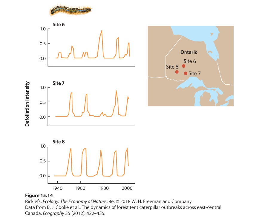
- Population Fluctuations in Nature
- Modeling Parasite and Host Populations
Ch 16CompetitionRead full chapter →
16Competition Garlic mustard is an invasive species that has spread throughout the eastern and midwestern United States. The invasive plant has a competitive advantage because it produces a toxin that harms native plants. Trying to Catch Up to Garlic Mustard Garlic mustard is a powerful forest foe. It was introduced to the United States from Europe 150 years ago and has since spread throughout eastern and midwestern forests. It not only spreads, it dominates as a competitor against native plant species. Where you find garlic mustard, you often find few other forest herbs. During the past decad…
mustard is a highly effective competitor because it possesses a novel weapon. However, its competitive advantage continues to evolve as it experiences changes in the intensity of competition from native plants, while the native plants continue to coevolve to combat the invader. “Garlic mustard is a highly effective competitor because it possesses a novel weapon.” SOURCES: Evans, J. A., et al. 2016. Soil-mediated eco-evolutionary feedbacks in the invasive plant Alliaria petiolata. Functional Ecology 30: 1053–1061. Lankau, R. A. 2012. Coevolution between invasive and native plants driven by chem…
Sections in this chapter
- 16 Competition
- Learning Objectives
- The Role of Resources
- The Competitive Exclusion Principle
- Concept Check
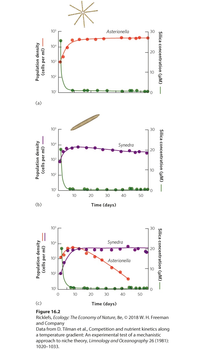
- Competition for A Single Resource
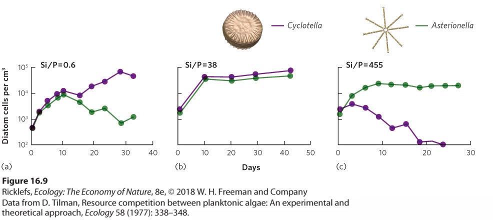
- Competition for Multiple Resources
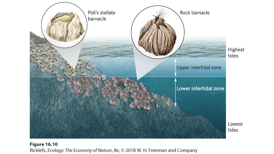
- Abiotic Conditions
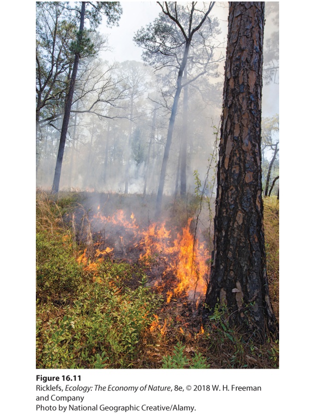
- Disturbances
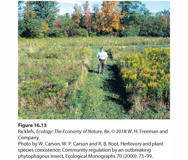
- Predation and Herbivory
- Apparent Competition
- Analyzing Ecology
Ch 17MutualismRead full chapter →
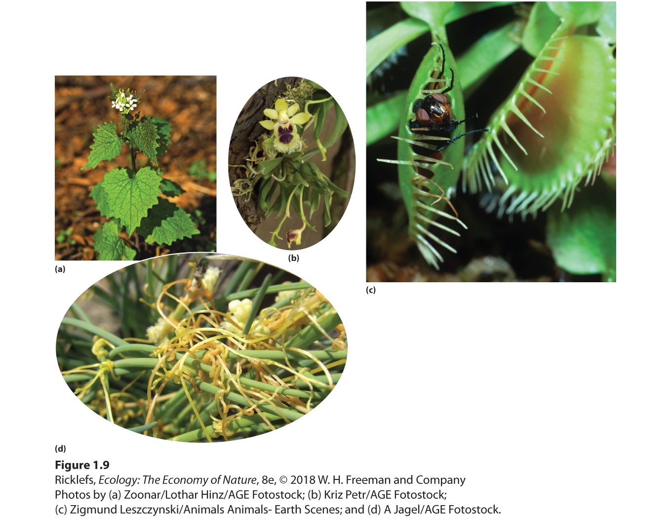
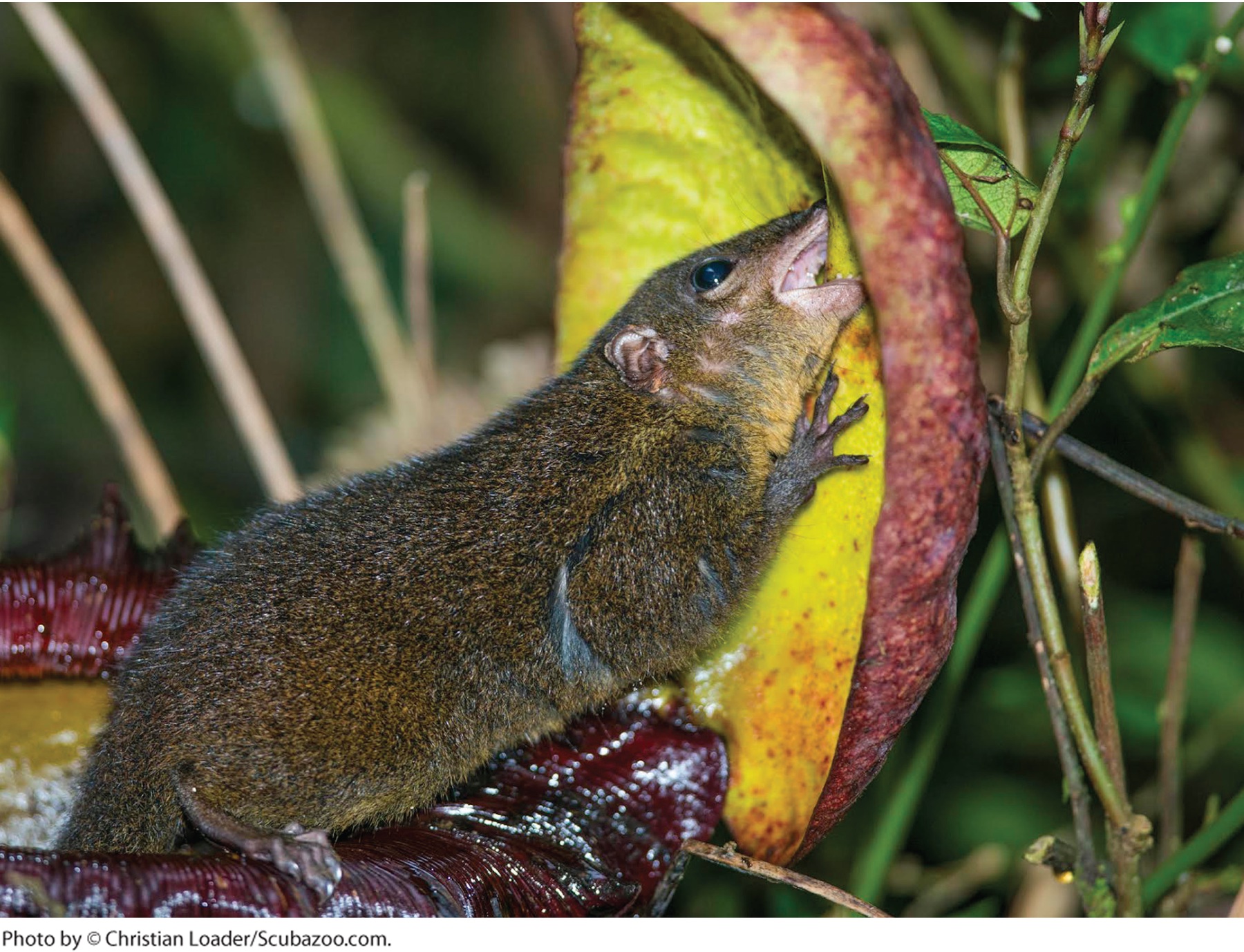
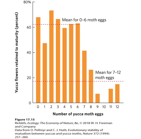
17Mutualism A tree shrew feeding on a pitcher plant in Borneo. The tree shrew consumes nectar from the plant and then defecates into the pitcher, which provides nitrogen-rich nutrients to the plant. Bathrooms with Benefits Pitcher plants are famous for trapping insects, which are attracted by the smell and the nectar produced by the plant. Unfortunately for the insects, the cup-shaped pitcher has a slippery rim, making it nearly impossible for insects to escape once they enter. As a result, the insects die and are subsequently digested by the plant. Through this predator–prey relationship, pit…
Sections in this chapter
- 17 Mutualism
- Learning Objectives
- Resource Acquisition in Plants
- Resource Acquisition in Animals
- Concept Check
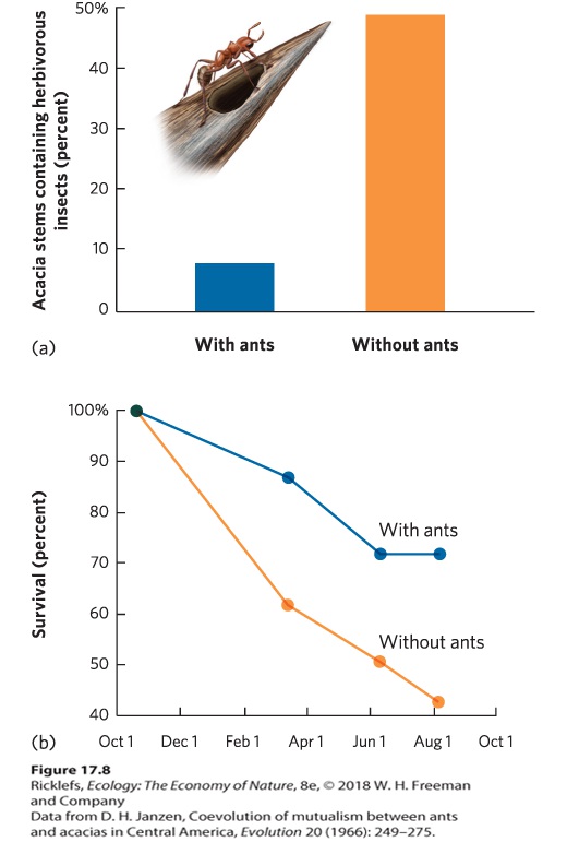
- Plant Defense
- Animal Defense
- Pollination
- Seed Dispersal
- Shifting from Mutualism to Negative Interactions
- Dealing with Cheaters in Mutualisms
- Effects on Species Distributions

Ch 18Community StructureRead full chapter →
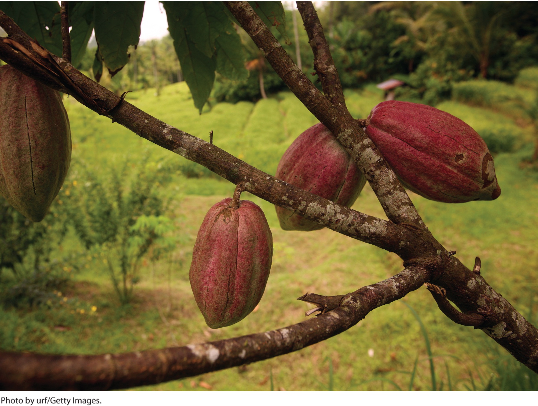
18Community Structure Cacao trees produce fruits that contain the cocoa beans. When old fruit husks are placed around the trees, they provide a habitat for the eggs and larvae of midges, which later turn into adult flies that pollinate the flowers of the cacao tree. Pollinating the “Food of the Gods” Chocolate is one of the most popular food ingredients in modern cuisines. It comes from the beans of the cacao tree (Theobroma cacao) that originated in South and Central America. Given that ancient people used it in religious ceremonies as gifts to their gods, the genus of the plants, Theobroma, …
cacao flowers and provides insect prey for multiple species of predators. Because these decomposing husks can also serve as a habitat for fungal pathogens that are harmful to cacao trees, the researchers suggest that other sources of decomposing plant matter, such as old banana stems, might be a better way of providing midge habitat while reducing the prevalence of the fungal pathogen. This research illuminates how ecological communities are made up of interconnected species and that these connections have a major impact on natural and agricultural communities. “By cleaning up the ground aroun…
Sections in this chapter
- 18 Community Structure
- Learning Objectives
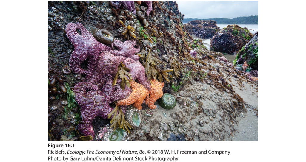
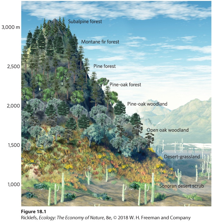
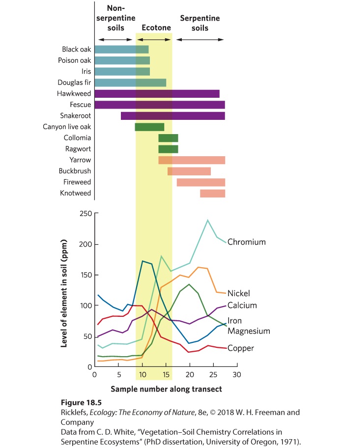
- Community Zonation
- Categorizing Communities
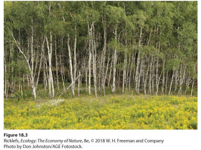
- Ecotones
- Independent Species Distributions
- Concept Check
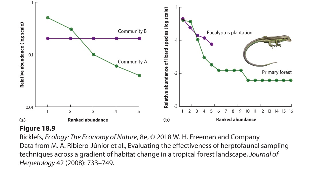
- Patterns of Abundance Among Species
- Rank-Abundance Curves
- Resources
- Analyzing Ecology
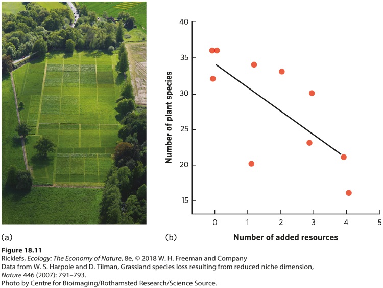
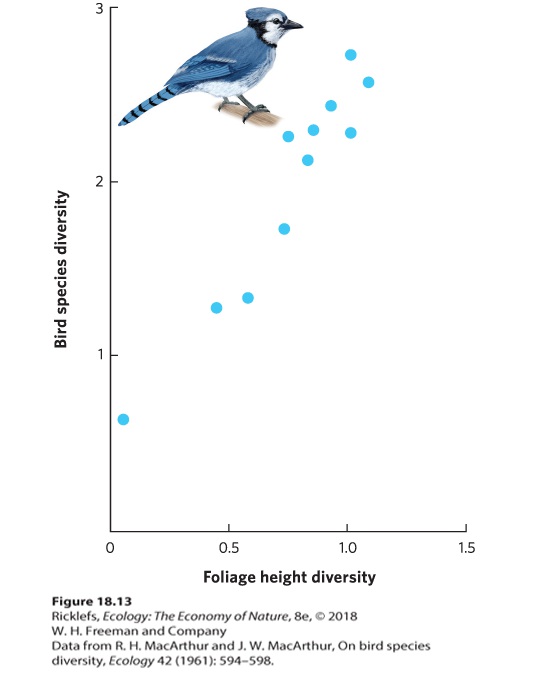
- Habitat Diversity
Ch 19Community SuccessionRead full chapter →
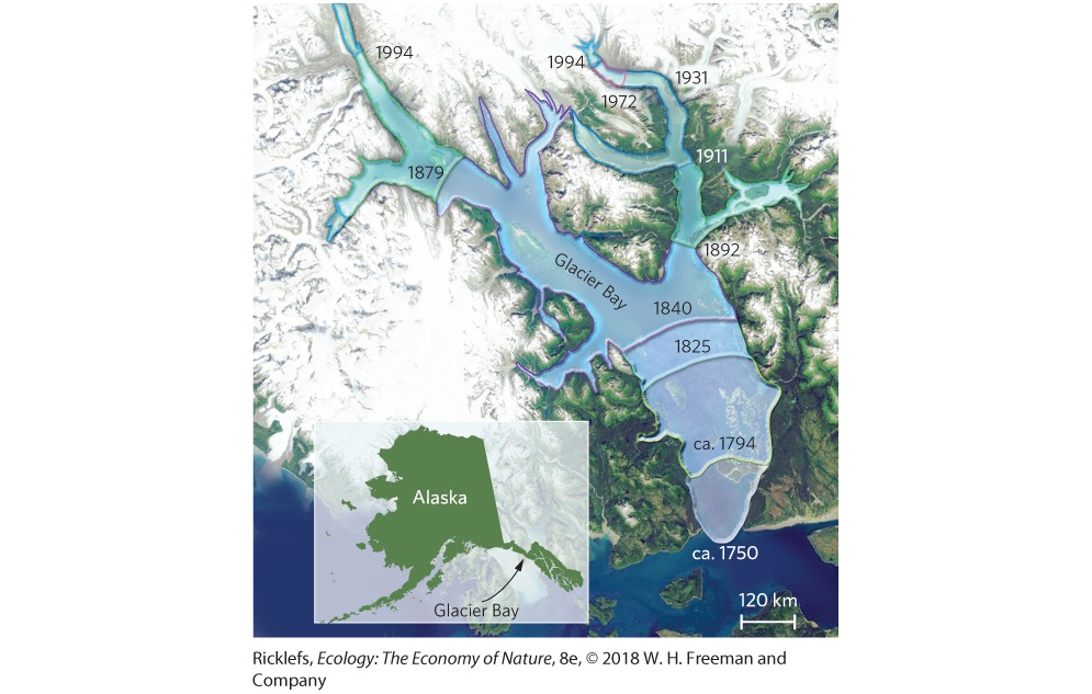
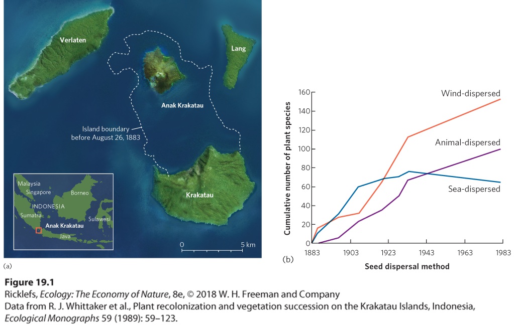
19Community Succession Glacier Bay, Alaska. In 1794, a glacier that was more than 1,200 m thick covered all but the inlet of the bay. Since then, the glaciers have melted and retreated, leaving behind a large body of water. Retreating Glaciers in Alaska In the panhandle of Alaska near Juneau, a stretch of land has undergone incredible changes during the past 200 years. In 1794, Captain George Vancouver found an inlet that headed toward modern-day Juneau. To the north of the inlet was a massive glacier that measured more than 1 km thick and 32 km wide. When the naturalist John Muir visited the …
The observations of Vancouver, Muir, and Cooper paved the way for more than a century of subsequent ecological research at Glacier Bay. In fact, the original terrestrial quadrats set up by Cooper a century ago are still monitored today, as are local streams that have been created by the melting glacier. Researchers are also examining the soils and finding that as the plant communities shift from mosses to shrubs to trees, the soil becomes more nutrient rich. As a result, they found that forbs and grasses grow better in soils containing more nutrients. As we will see in this chapter, long-term …
Sections in this chapter
- 19 Community Succession
- Learning Objectives
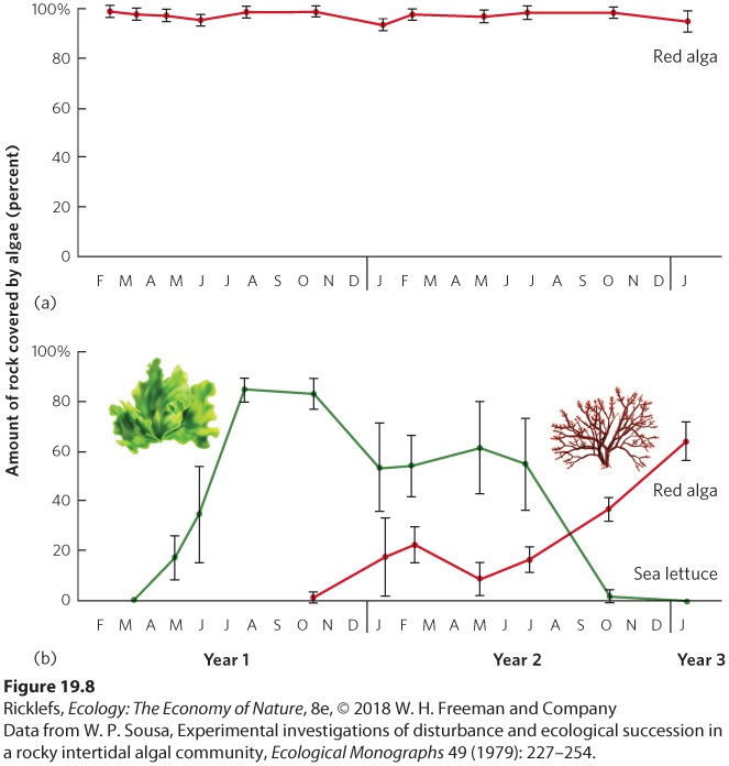
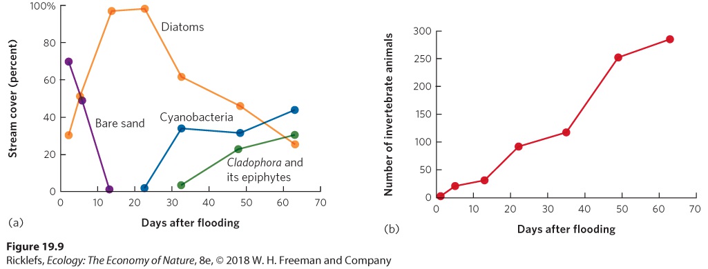
- Observing Succession
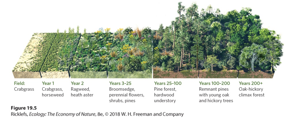
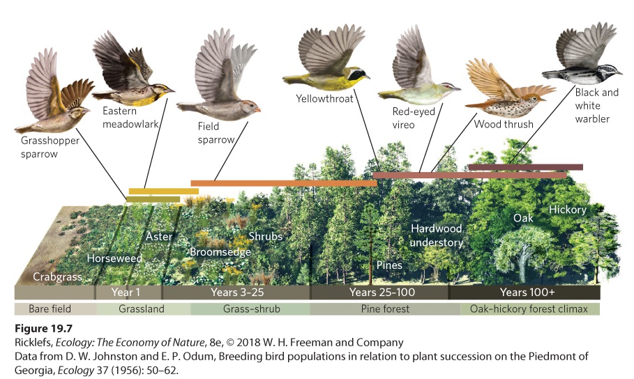
- Succession in Terrestrial Environments
- Succession in Aquatic Environments
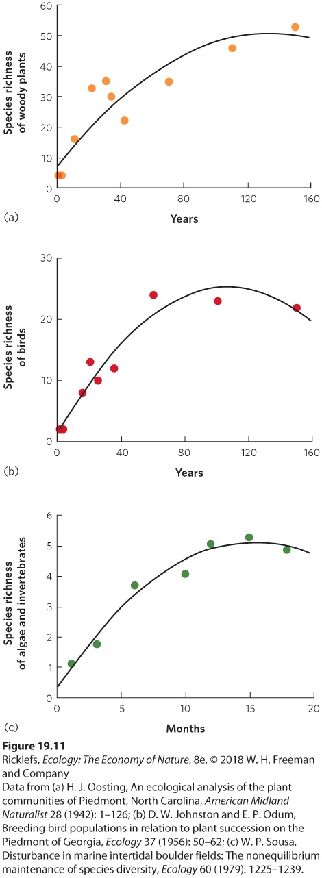
- Change in Species Diversity
- Concept Check
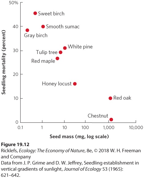
- Traits of Early- Versus Late-Succession Species
- Analyzing Ecology
- Facilitation, Inhibition, and Tolerance
- Tests for the Mechanisms of Succession
- Changes in Climax Communities over Time

Ch 20Movement of Energy in EcosystemsRead full chapter →
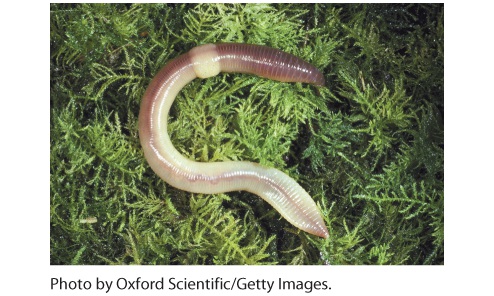
20Movement of Energy in Ecosystems The red-backed salamander. The introduction of earthworms from Europe and Asia to northern forests that historically lacked earthworms has caused a decline in leaf litter and soil insects. This has led to a sharp decline in the abundance of red-backed salamanders. Worming Your Way into an Ecosystem Earthworms play an important role in terrestrial ecosystems. As they burrow in the ground to consume detritus, they aerate compact soils, which allows water to better percolate into the ground. Earthworms seem to be everywhere in North America; you may have seen th…
Sections in this chapter
- 20 Movement of Energy in Ecosystems
- Learning Objectives
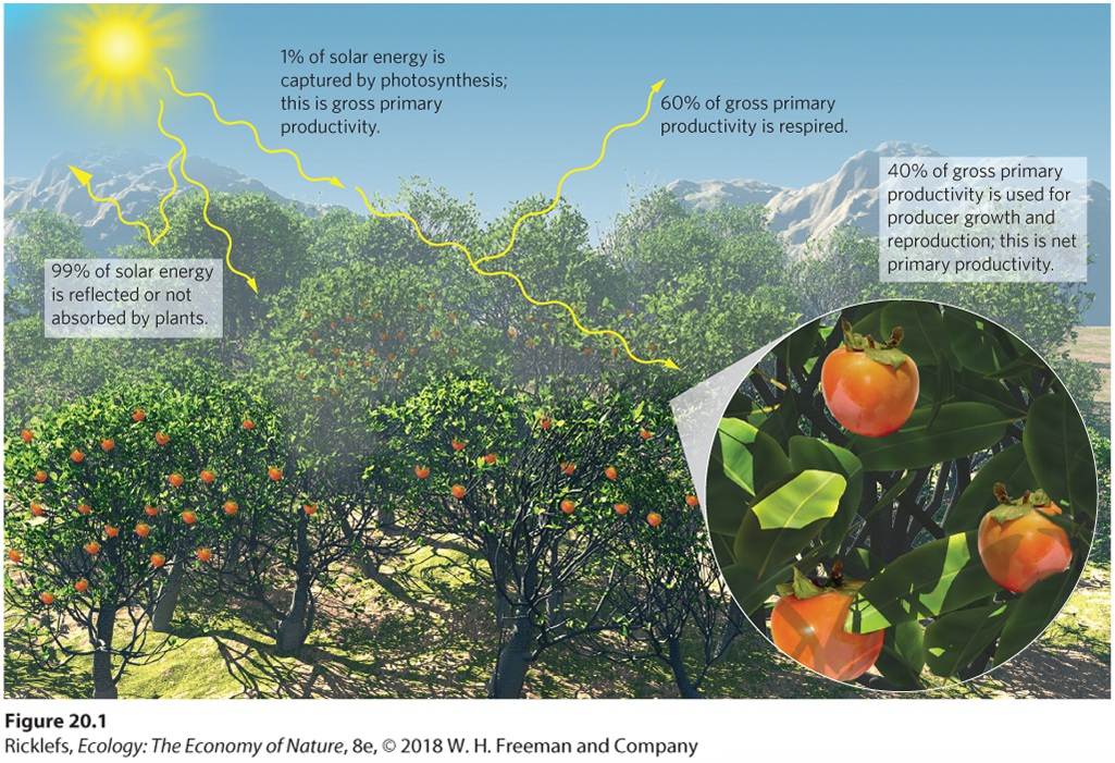
- Primary Productivity
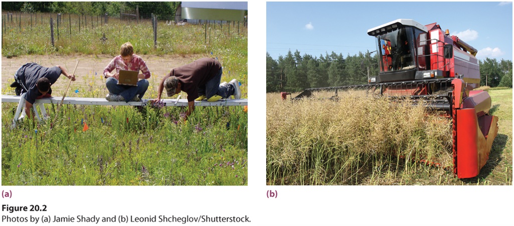
- Measuring Primary Productivity
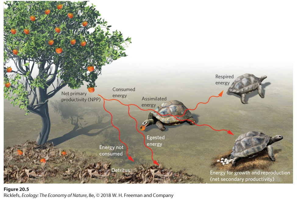
- Secondary Production
- Concept Check
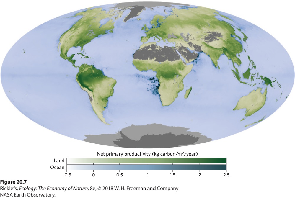
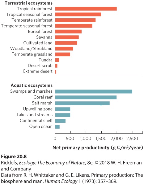
- Primary Productivity Around the World
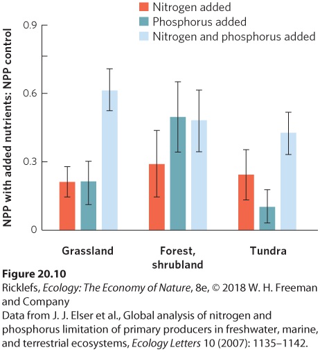
- Drivers of Productivity in Terrestrial Ecosystems
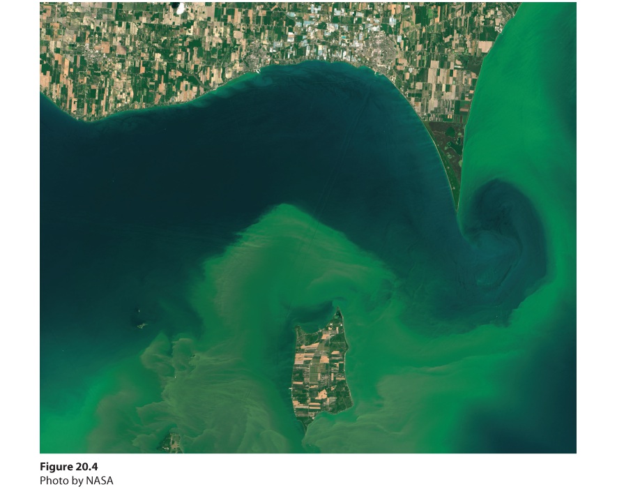
- Drivers of Productivity in Aquatic Ecosystems
- Trophic Pyramids
- The Efficiencies of Energy Transfers
- Analyzing Ecology
Ch 21Movement of Elements in EcosystemsRead full chapter →
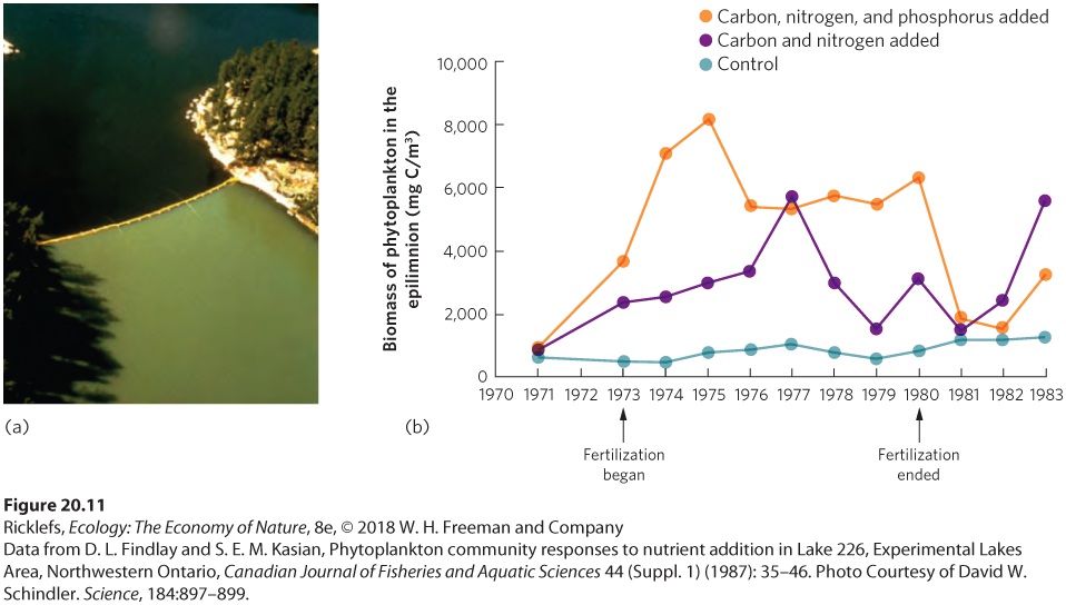
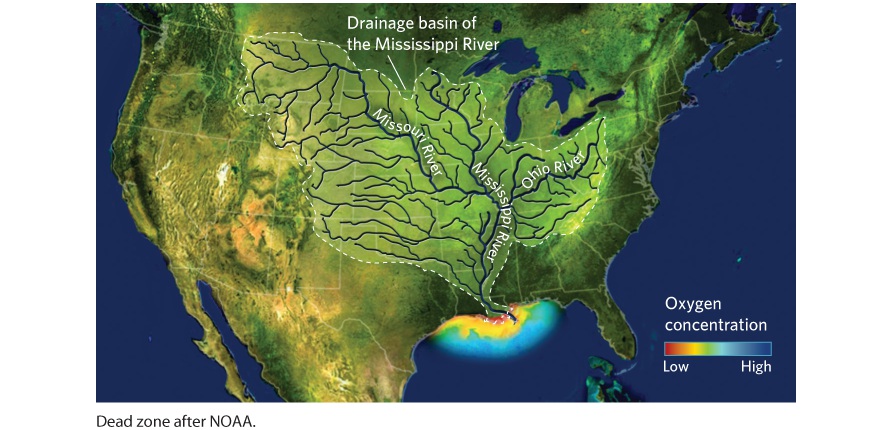
21Movement of Elements in Ecosystems The effects of a dead zone on fish populations. Because algae that bloom will eventually die, the decomposition uses up nearly all the oxygen in the water. These fish died from a dead zone that occurred in Lake Trafford, Florida. Living in a Dead Zone Each summer, as the Mississippi River flows into the Gulf of Mexico, an area develops where animals can’t survive. While fish, crawfish, and crabs remain abundant in other parts of the Gulf, the summer algal bloom in this area makes it uninhabitable. In many cases, the rapidly increasing populations of algae c…
Sections in this chapter
- 21 Movement of Elements in Ecosystems
- Learning Objectives
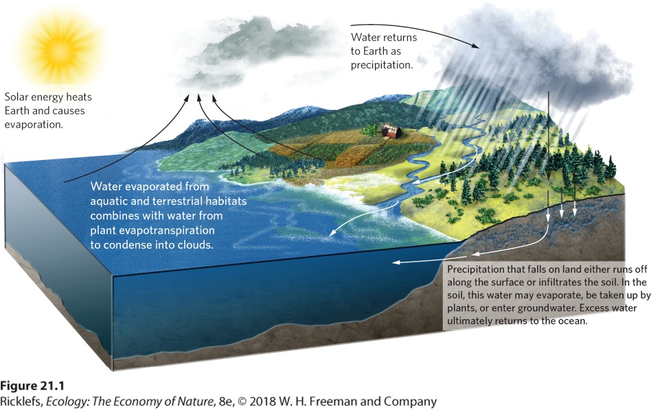
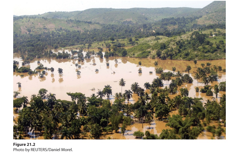
- The Hydrologic Cycle
- Human Impacts on the Hydrologic Cycle
- Concept Check
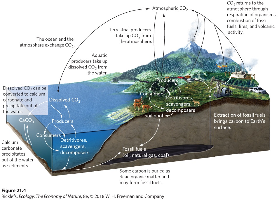
- The Carbon Cycle
- Human Impacts on the Carbon Cycle
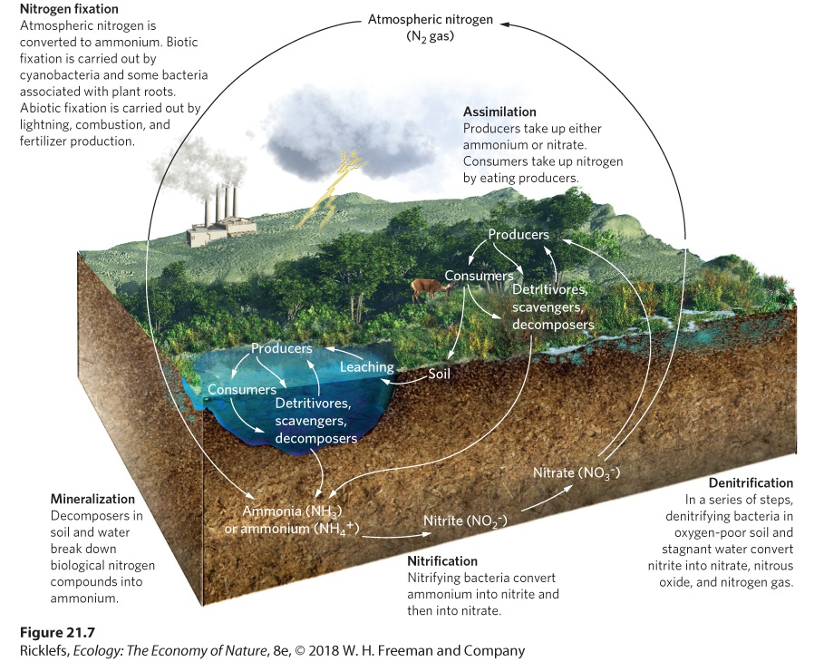
- The Nitrogen Cycle
- Human Impacts on the Nitrogen Cycle
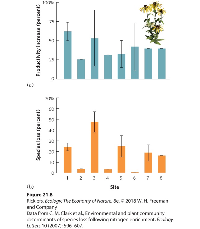
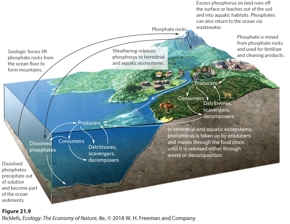
- The Phosphorus Cycle
- Human Impacts on the Phosphorus Cycle
- The Importance of Weathering
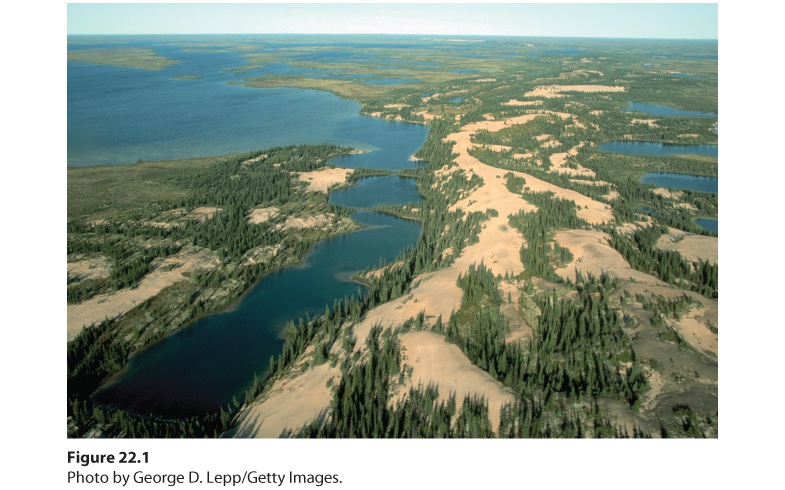
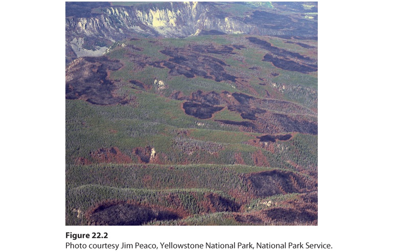
Ch 22Landscape Ecology and Global BiodiversityRead full chapter →
22Landscape Ecology and Global Biodiversity Species diversity of flowering plants in California. While California has experienced 28 extinctions of native plants, they have also experienced introductions of more than 1,000 nonnative plants from around the world. Can We Have Too Much Biodiversity? The word biodiversity prompts several thoughts. We think of the diversity of evolved species that play unique roles in nature and collectively contribute to the proper functioning of ecosystems. We also may think about the many species around the world that are declining in abundance and some that are…
Sections in this chapter
- 22 Landscape Ecology and Global Biodiversity
- Learning Objectives
- Causes of Habitat Heterogeneity
- Species Diversity
- Local and Regional Species Diversity
- Concept Check
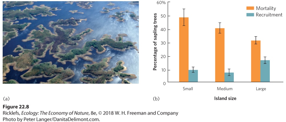
- Habitat Fragmentation
- Analyzing Ecology
- Dragonflies
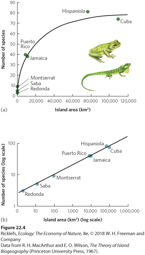
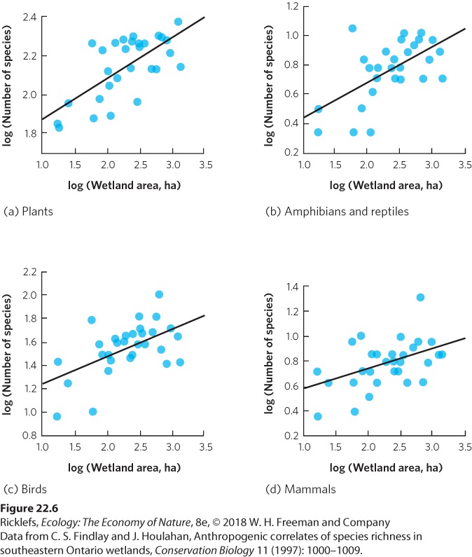
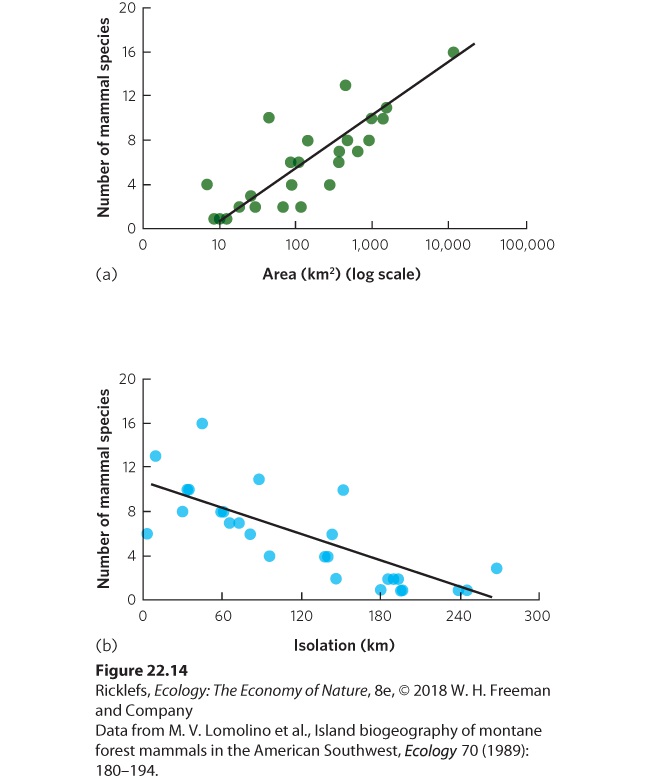
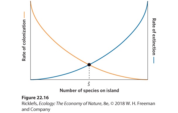
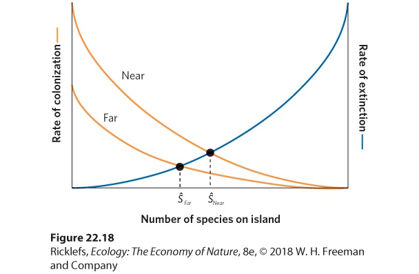
- The Evidence
- The Theory
- Reserves
Ch 23Conservation of Global BiodiversityRead full chapter →
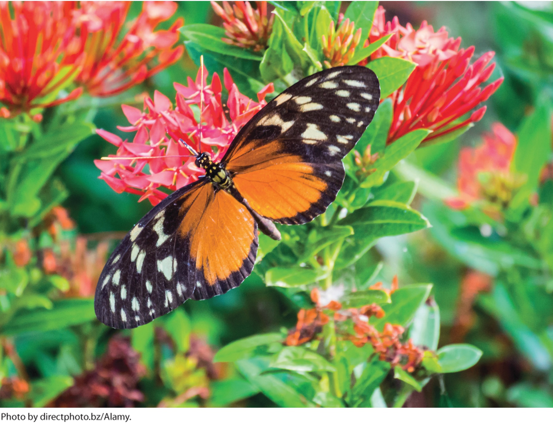
23Conservation of Global Biodiversity Conserving biodiversity. Efforts are being made to protect the world’s biodiversity, including this tiger longwing butterfly (Heliconius ismenius) from Costa Rica. Protecting Hotspots of Biodiversity The biodiversity of the world faces a wide range of threats from a growing human population that has caused species to go extinct at a rapid rate. To reverse this downward spiral, conservationists seek ways to protect aquatic and terrestrial ecosystems so that threats from human activities can be reduced or eliminated. A common approach to protecting species i…
Sections in this chapter
- 23 Conservation of Global Biodiversity
- Learning Objectives
- Instrumental Values
- Intrinsic Values
- Concept Check
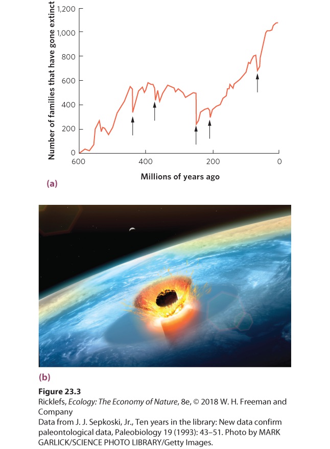
- Background Extinction Rates
- A Possible Sixth Mass Extinction
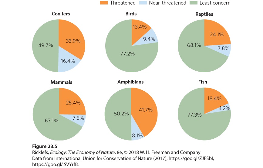
- Global Declines in Species Diversity
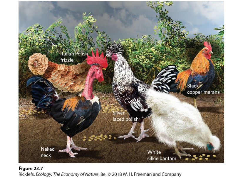
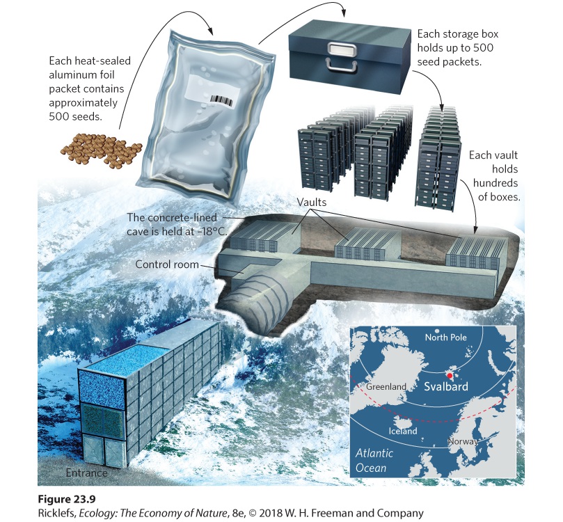
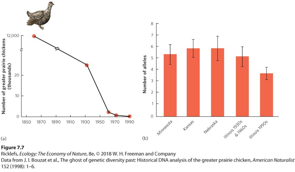
- Global Declines in Genetic Diversity
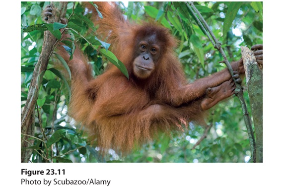
- Habitat Loss
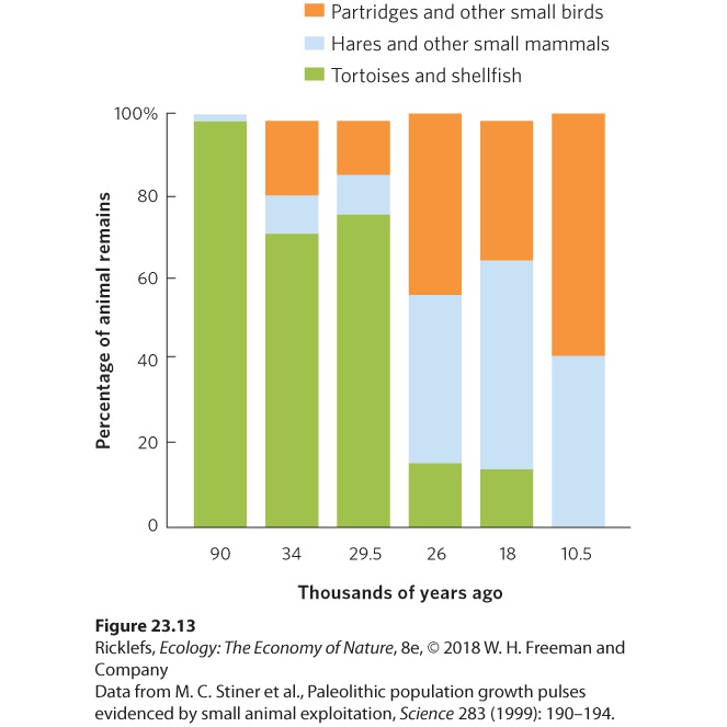
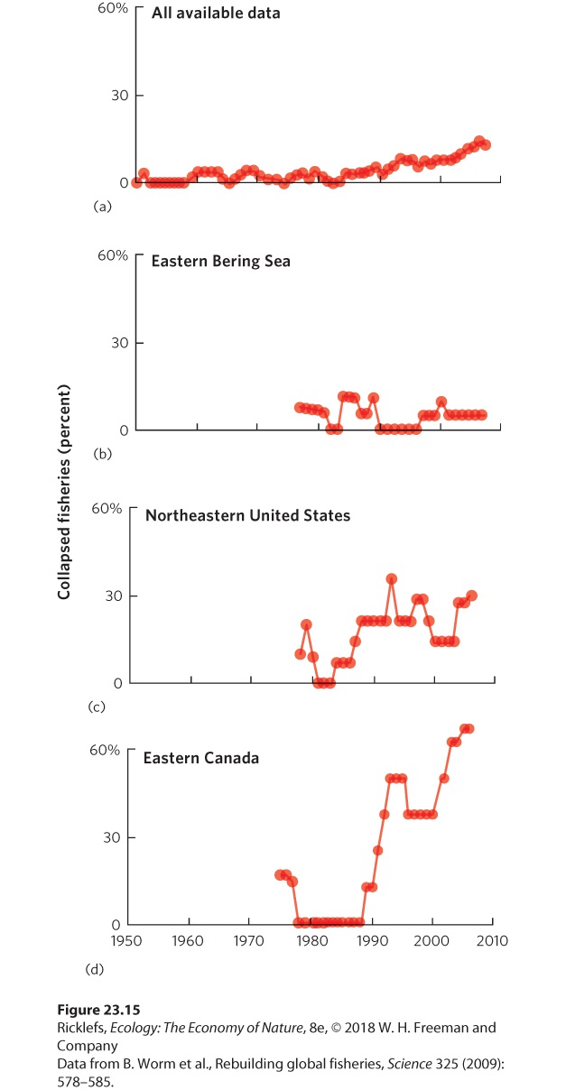
- Overharvesting
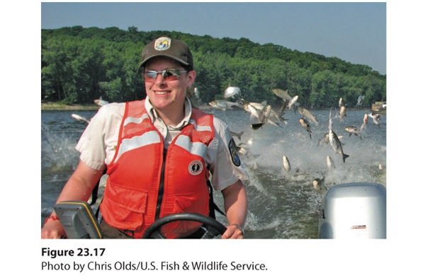
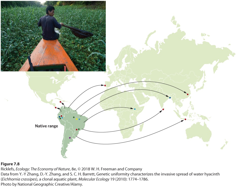
- Introduced Species