Chapter 12: Data-Based and Statistical Reasoning

Chapter 12: Data-Based and Statistical Reasoning
Science Mastery Assessment
Every pre-med knows this feeling: there is so much content I have to know for the MCAT! How do I know what to do first or what’s important?
While the high-yield badges throughout this book will help you identify the most important topics, this Science Mastery Assessment is another tool in your MCAT prep arsenal. This quiz (which can also be taken in your online resources) and the guidance below will help ensure that you are spending the appropriate amount of time on this chapter based on your personal strengths and weaknesses. Don’t worry though— skipping something now does not mean you’ll never study it. Later on in your prep, as you complete full-length tests, you’ll uncover specific pieces of content that you need to review and can come back to these chapters as appropriate.
How to Use This Assessment
If you answer 0–7 questions correctly:
Spend about 1 hour to read this chapter in full and take limited notes throughout. Follow up by reviewing all quiz questions to ensure that you now understand how to solve each one.
If you answer 8–11 questions correctly:
Spend 20–40 minutes reviewing the quiz questions. Beginning with the questions you missed, read and take notes on the corresponding subchapters. For questions you answered correctly, ensure your thinking matches that of the explanation and you understand why each choice was correct or incorrect.
If you answer 12–15 questions correctly:
Spend less than 20 minutes reviewing all questions from the quiz. If you missed any, then include a quick read-through of the corresponding subchapters, or even just the relevant content within a subchapter, as part of your question review. For questions you got correct, ensure your thinking matches that of the explanation and review the Concept Summary at the end of the chapter.
- The inclusion of an outlier in statistical analysis will most greatly affect which of the following measurements?
- Median
- Mode
- Mean
- All three are equally affected
- In a sample of hospital patients, the mean age is found to be significantly lower than the median. Which of the following best describes this distribution?
- Skewed right
- Skewed left
- Normal
- Bimodal
- What is the median of the following data set?
7, 17, 53, 23, 4, 2, 4
- 4
- 7
- 15.7
- 23
- On Santa Cruz island, the available food sources led to disruptive selection in the beak sizes of finches, in which large and small beak sizes were favored over intermediate sized beaks. As a result, few finches have an intermediate sized beak. If a sample of finches were analyzed, what distribution would best describe the distribution of beak size?
- Normal
- Bimodal
- Skewed left
- Skewed right
- A 95% confidence interval will fall within what distance from the mean?
- ±σ
- ±2σ
- ±3σ
- ±4σ
- Approximately 20% of people who live in the United States eat fast food at least once per week. A new study conducted by the National Heart Association showed that 48% of US residents have some form of cardiovascular disease. Which of the following hypothetical findings could be used to show that cardiovascular disease is independent of weekly fast food consumption?
- Individuals who do not consume fast food do not have cardiovascular disease.
- Of the 48% of those who had cardiovascular disease, only half of them ate fast food on a weekly basis.
- 9.6% of US residents have cardiovascular disease and consume fast food on a weekly basis.
- None of the individuals who consume fast food on a weekly basis develop cardiovascular disease.
- Which of the following outliers would most likely be the easiest to correct?
- A typographical error in data transfer
- A measurement error in instrument calibration
- A heavily skewed distribution
- A correctly measured anomalous result
- Assume that blonde hair and blue eyes are independent recessive traits. If one parent is a carrier for each gene while the other parent is homozygous recessive for both genes, what is the probability that the first two offspring will both have blonde hair and blue eyes?
- 6.25%
- 25%
- 43.75%
- 50%
- Based on the county-level map below, which of the following statements best represents the data about individuals older than 65 in the continental United States? (Note: The darker the shade of green, the higher the percentage of persons over 65 in the county.)

- Most of the people over 65 in the United States live in the center of the country.
- Most of the people living in the center of the United States are over 65.
- The center of the United States tends to have a larger proportion of people over 65.
- There are more people over 65 moving to the center of the country than elsewhere.
- As the confidence level increases, a confidence interval:
- becomes wider.
- becomes thinner.
- shifts to higher values.
- shifts to lower values.
- Which of the following measures of distribution is most useful for determining probabilities?
- Range
- Average distance from mean
- Interquartile range
- Standard deviation
- Are there any outliers on the following box plot?
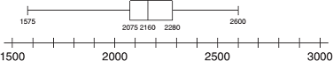
- Yes; 1575 is an outlier.
- Yes; 2600 is an outlier.
- Yes; both 1575 and 2600 are outliers.
- No; there are no outliers.
- A gas station attendant notices that there are more assaults near the station on the days that a lot of ice cream is sold and hypothesizes that the ingestion of excess glucose leads to an increase in violent behavior. The attendant begins to tally how much ice cream is sold on a daily basis and checks the daily crime statistics to generate the graph below.
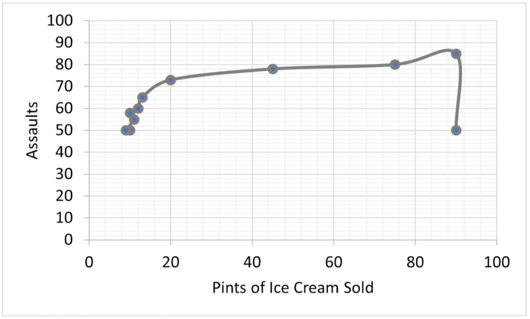
The attendant analyzes the data and concludes that the hypothesis is true. Are there any flaws in this conclusion?
- No, the number of assaults increases as the pints of ice cream sold increase.
- No, the study is appropriately controlled.
- Yes, the study is missing a positive control.
- Yes, the attendant has proved correlation, but not a causal link.
- The following histogram:
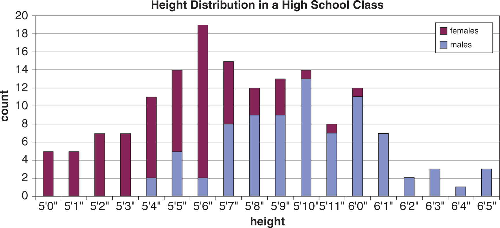
- contains a bimodal distribution.
- should be analyzed as two separate distributions.
- contains one mode.
- II only
- I and II only
- I and III only
- I, II, and III
- A cardiologist is investigating a new drug therapy for the treatment of hypertension. The cardiologist measures the baseline blood pressure of several patients, then treats them with the drug for ten weeks, measuring their blood pressure again after this time.
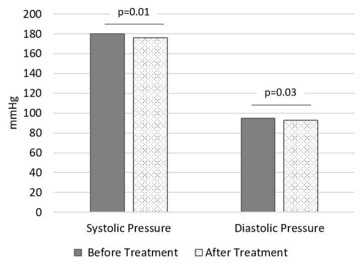
Based on these data, should the doctor advocate for making this drug the standard treatment for hypertension?
- Yes, there is a statistically significant decrease in blood pressure.
- Yes, the drug is effective at decreasing blood pressure.
- No, while statistically significant, the results are not clinically significant.
- No, the data is not statistically significant.
Answer Key
- C
- B
- B
- B
- B
- C
- A
- A
- C
- A
- D
- C
- D
- D
- C
Chapter 12: Data-Based and Statistical Reasoning
CHAPTER 12
DATA-BASED AND STATISTICAL REASONING
In This Chapter
12.1 Measures of Central Tendency
Mean
Median
Mode
12.2 Distributions
Normal Distributions
Skewed Distributions
Bimodal Distributions
12.3 Measures of Distribution
Range
Interquartile Range
Standard Deviation
Outliers
12.4 Probability
Independence, Mutual Exclusivity, and Exhaustiveness
Calculations
12.5 Statistical Testing
Hypothesis Testing
Confidence Intervals
12.6 Charts, Graphs, and Tables
Types of Charts
Graphs and Axes
Interpreting Tables
12.7 Applying Data
Correlation and Causation
In the Context of Scientific Knowledge
Concept Summary
MCAT EXPERTISE
Chapter 12 does not contain a chapter profile as it does not directly cover any AAMC content categories. That said, just like with Chapter 11 of this book, the AAMC has confirmed that 10% of the science questions on every MCAT will require material in this chapter—and many of those questions will require only information from this chapter, without any other supportive science content. With 10% from Chapter 11 and 10% from Chapter 12, there will be more than 30 questions(!) on your exam that will test one of these two skills.
Introduction
Academic papers are extremely predictable. They generally begin with an abstract that reflects the major points of the rest of the paper. The authors then provide an expanded introduction, materials and methods, data, and discussion. The key to a high-quality research paper is making this discussion unnecessary—any scientists, when given the prior sections, should be led to the same conclusions as those given by the author. The testmakers are keenly aware of this fact. On Test Day, you may be presented with research in the form of an experiment-based passage and part of your task will be inferring the important conclusions that can be supported by the findings of the study.
This chapter covers the last of the Scientific Inquiry and Reasoning Skills tested on the MCAT: the statistical analysis of raw data, interpretation of visual representations of this data, and application of data to answer research questions. We’ll begin by examining basic statistical principles like distribution types, measures of central tendency, and measures of distribution. We’ll also discuss probability, and the semantics of this branch of mathematics. We’ll conclude our discussion of probability and statistics with an exploration of statistical significance in basic hypothesis testing and confidence intervals. Then, we’ll move on to the interpretation of charts and graphs. Finally, we’ll link all of this information with the skills we gained in the last chapter and assess the future use and validity of studies.
12.1 Measures of Central Tendency
LEARNING OBJECTIVES
After Chapter 12.1, you will be able to:
- Calculate mean, median, and mode for a data set
- Predict the best measure of central tendency for a given data set
Measures of central tendency are those that describe the middle of a sample. How we define middle can vary. Is it the mathematical average of the numbers in the data set? Is it the result in a data set that divides the set into two—with half the sample values above this result and half the sample values below? Both of these data can be important, and the difference between them can also provide useful information on the shape of a distribution.
Mean
The mean or average of a set of data (more accurately, the arithmetic mean) is calculated by adding up all of the individual values within the data set and dividing the result by the number of values:
x¯=∑i=1n xin
Equation 12.1
where *x**itox**nare the values of all of the data points in the set andn* is the number of data points in the set. As we discussed in the last chapter, the mean may be a parameter or a statistic (as is true of all of the measures of central tendency) depending on whether we are discussing a population or a sample. Mean values are a good indicator of central tendency when all of the values tend to be fairly close to one another. Having an outlier—an extremely large or extremely small value compared to the other data values—can shift the mean toward one end of the range. For example, the average income in the United States is about $70,000, but half of the population makes less than $50,000. In this case, the small number of extremely high-income individuals in the distribution shifts the mean to the high end of the range.
Example: The following data were collected on the ages of attendees at Ray’s birthday party:
23, 22, 25, 22, 22, 24, 36, 20
What is the mean age of the attendees? Is this an appropriate measure for this data?
Solution: The mean is the sum of the data points divided by the number of data points:
x¯=23+22+25+22+22+24+36+208=1948=24.25
Because the mean is relatively near most of the values collected for this data set, it may be appropriate. Keep in mind, though, that the presence of an outlier and the fact that the mean is greater than all but two of the values collected indicates that the mean has been shifted toward the high end of the range. The presence of a single outlier does not invalidate the mean, but it does make interpretation in context necessary.
Median
The median value for a set of data is its midpoint, where half of data points are greater than the value and half are smaller. In data sets with an odd number of values, the median will actually be one of the data points. In data sets with an even number of values, the median will be the mean of the two central data points. To calculate the median, a data set must first be listed in increasing fashion. The position of the median can be calculated as follows:
median position=(n+1)2
Equation 12.2
where n is the number of data values. In a data set with an even number of data points, this equation will solve for a noninteger number; for example, in a data set with 18 points, it will be 18+12=9.5. The median in this case will be the arithmetic mean of the ninth and tenth items in the data set when sorted in ascending order.
The median tends to be the least susceptible to outliers, but may not be useful for data sets with very large ranges (the distance between the largest and smallest data point, as discussed later in this chapter) or multiple modes.
Example: Using the same data from the last question, find the median age of the attendees. Comparing this value to the mean, is the median a better or worse indicator of central tendency in this sample?
Solution: The first step in finding the median is to order the data from smallest to largest. Our original data was:
23, 22, 25, 22, 22, 24, 36, 20
Reordered, this becomes:
20, 22, 22, 22, 23, 24, 25, 36
n, the number of data points, is 8, so the median will be the average of the fourth and fifth data points. The median is therefore 22+232=22.5. The median is a better indicator of central tendency for this data than the mean of 24.25. The median is unaffected by the outlier and lies close to most of the values in the data set. One could improve the representativeness of the mean by excluding 36 from the data set, in which case the mean would be 22.6 while the median would be 22.
If the mean and the median are far from each other, this implies the presence of outliers or a skewed distribution, as discussed later in this chapter. If the mean and median are very close, this implies a symmetrical distribution.
KEY CONCEPT
The median divides the data set into two groups with 50% of values higher than the median and 50% of values lower than it.
Mode
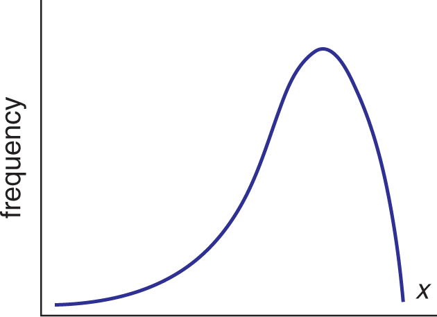
The mode, quite simply, is the number that appears the most often in a set of data. There may be multiple modes in a data set, or—if all numbers appear equally—there can even be no mode for a data set. When we examine distributions, the peaks represent modes. The mode is not typically used as a measure of central tendency for a set of data, but the number of modes, and their distance from one another, is often informative. If a data set has two modes with a small number of values between them, it may be useful to analyze these portions separately or to look for other variables that may be responsible for dividing the distribution into two parts.
MCAT CONCEPT CHECK 12.1
Before you move on, assess your understanding of the material with these questions.
- What types of data sets are best analyzed using the mean as a measure of central tendency?
_________________________________
_________________________________
- Calculate the mean, median, and mode of the following data set:
25, 23, 23, 6, 9, 21, 4, 4, 2
- Mean:
_________________________________
- Median:
_________________________________
- Mode:
_________________________________
12.2 Distributions
LEARNING OBJECTIVES
After Chapter 12.2, you will be able to:
- Assess whether data without a normal distribution can be analyzed with measures of central tendency and distribution
- Distinguish between normal, skewed, and bimodal distributions
- Describe the relationship between mean, median, and mode in different types of distributions:
Often a single statistic for a data set is insufficient for a detailed or relevant analysis. In this case, it is useful to look at the overall shape of the distribution as well as specifics about how that shape impacts our interpretation of the data. The shape of a distribution will impact all of the measures of central tendency that we have already discussed, as well as some measures of distribution, which we will examine later.
Normal Distributions
In statistics, we most often work with a normal distribution, shown in Figure 12.1. Even when we know that this is not quite the case, we can use special techniques so that our data will approximate a normal distribution. This is very important because the normal distribution has been “solved” in the sense that we can transform any normal distribution to a standard distribution with a mean of zero and a standard deviation of one, and then use the newly generated curve to get information about probability or percentages of populations. The normal distribution is also the basis for the bell curve seen in many scenarios, including exam scores on the MCAT.
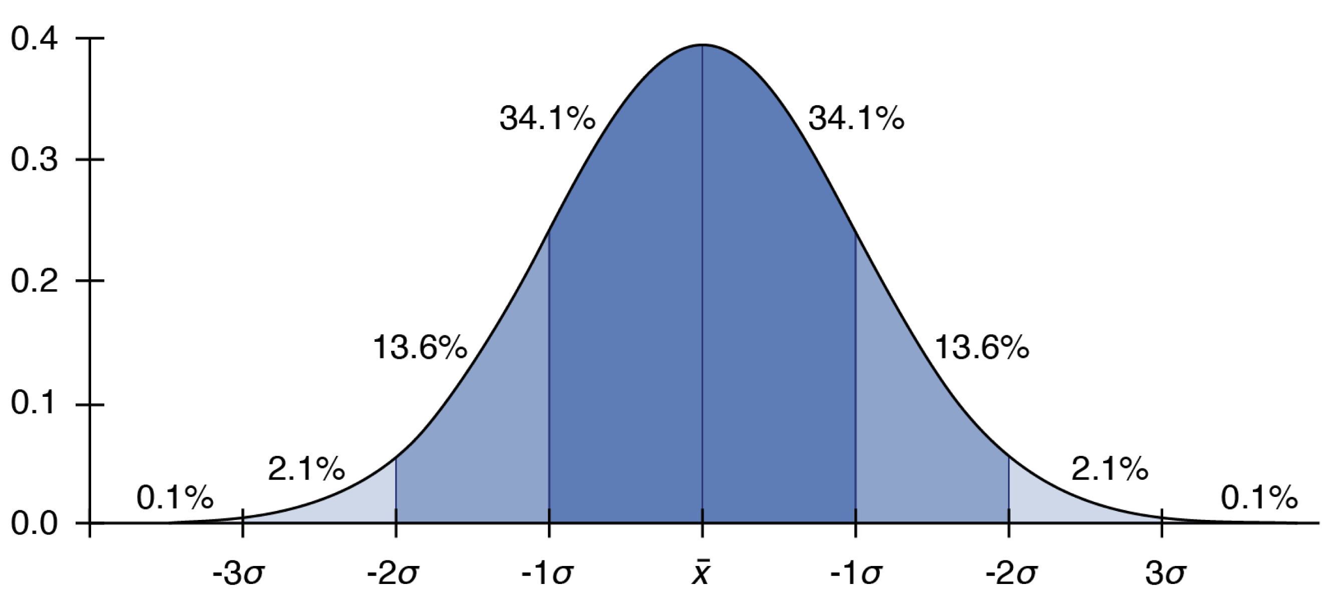
Figure 12.1. The Normal Distribution The mean, median, and mode are at the center of the distribution. Approximately 68% of the distribution is within one standard deviation of the mean, 95% within two, and 99% within three.
KEY CONCEPT
The normal distribution and its counterpart, the standard distribution, are the basis of most statistical testing on the MCAT. In the normal distribution, all of the measures of central tendency are the same.
Skewed Distributions
Distributions are not always symmetrical. A skewed distribution is one that contains a tail on one side or the other of the data set. On the MCAT, skewed distributions are most often tested by simply identifying their type. This is often an area of confusion for students because the visual shift in the data appear opposite the direction of the skew. A negatively skewed distribution has a tail on the left (or negative) side, whereas a positively skewed distribution has a tail on the right (or positive) side. Because the mean is more susceptible to outliers than the median, the mean of a negatively skewed distribution will be lower than the median, while the mean of a positively skewed distribution will be higher than the median. These distributions, and their measures of central tendency, are shown in Figure 12.2.
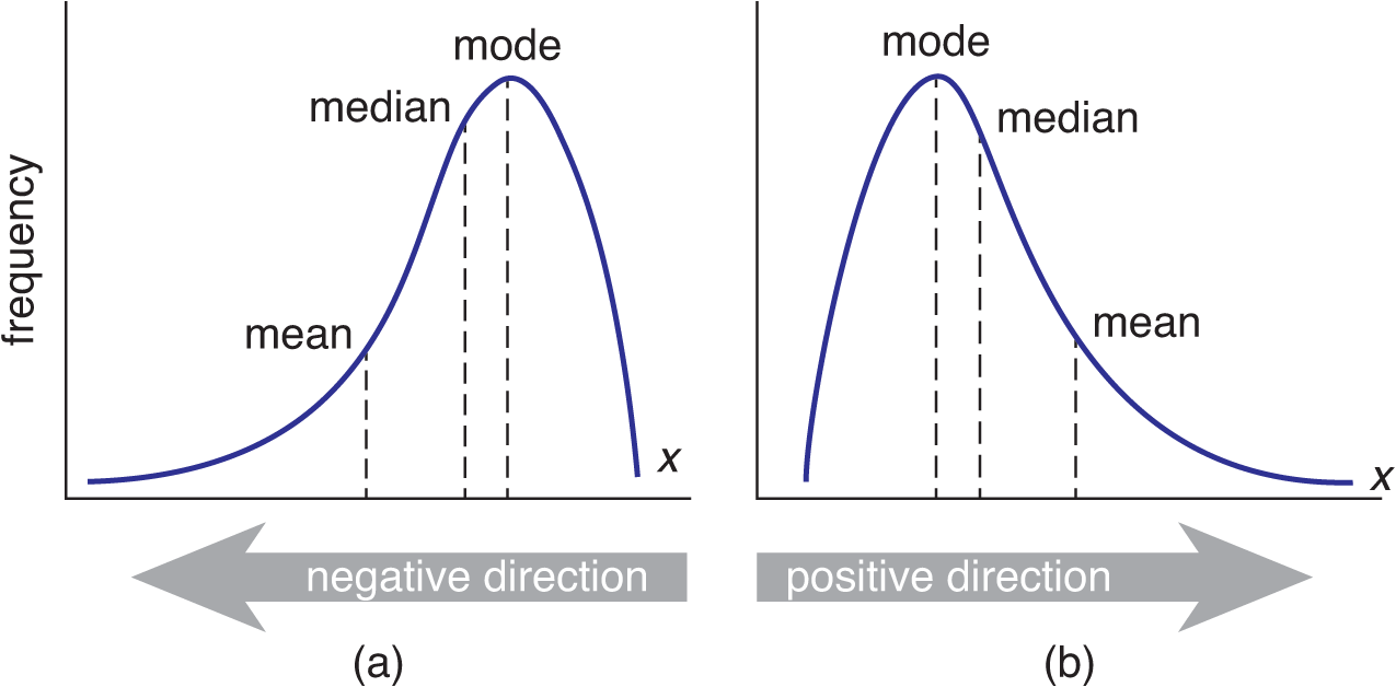
Figure 12.2. Skewed Distributions (a) Negatively skewed distribution, with mean lower than median; (b) Positively skewed distribution, with mean higher than median.
KEY CONCEPT
The direction of skew in a sample is determined by its tail, not the bulk of the distribution.
Bimodal Distributions
Some distributions have two or more peaks. A distribution containing two peaks with a valley in between is called bimodal, as shown in Figure 12.3. It is important to note that a bimodal distribution, strictly speaking, might have only one mode if one peak is slightly higher than the other. However, even when the peaks are of two different sizes, we still call the distribution bimodal. If there is sufficient separation of the two peaks, or a sufficiently small amount of data within the valley region, bimodal distributions can often be analyzed as two separate distributions. On the other hand, bimodal distributions do not have to be analyzed as two separate distributions either; the same measures of central tendency and measures of distribution can be applied to them as well.
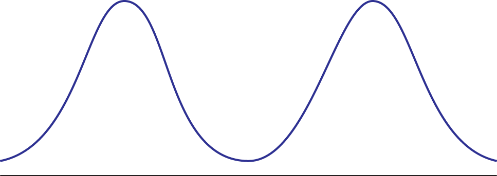
Figure 12.3. Bimodal Distribution
MCAT CONCEPT CHECK 12.2
Before you move on, assess your understanding of the material with these questions.
- How do the mean, median, and mode compare for a right-skewed distribution?
_________________________________
- Can data that do not follow a normal distribution be analyzed with measures of central tendency and measures of distribution? Why or why not?
_________________________________
- What is the difference between normal or skewed distributions, and bimodal distributions?
_________________________________
12.3 Measures of Distribution
LEARNING OBJECTIVES
After Chapter 12.3, you will be able to:
- Identify outliers using interquartile range or standard deviation
- Describe the relationship between range and standard deviation
- Justify whether certain measures of distribution are or are not appropriate for a given situation
Distributions can be characterized not only by their “center” points, but also by the spread of their data. This information can be described in a number of ways. Range is an absolute measure of the spread of a data set, while interquartile range and standard deviation provide more information about the distance that data falls from one of our measures of central tendency. We can use these quantities to determine if a data point is truly an outlier in our data set.
Range
The range of a data set is the difference between its largest and smallest values:
range = xmax − xmin
Equation 12.3
Range does not consider the number of items of the data set, nor does it consider the placement of any measures of central tendency. Range is therefore heavily affected by the presence of data outliers. In cases where it is not possible to calculate the standard deviation for a normal distribution because the entire data set is not provided, it is possible to approximate the standard deviation as one-fourth of the range.
Interquartile Range
Interquartile range is related to the median, first, and third quartiles. Quartiles, including the median (Q2), divide data (when placed in ascending order) into groups that comprise one-fourth of the entire set. There is some debate over the most appropriate way to calculate quartiles; for the purposes of the MCAT, we will use the most common (and simplest) method:
- To calculate the position of the first quartile (Q1) in a set of data sorted in ascending order, multiply n by 14.
- If this is a whole number, the quartile is the mean of the value at this position and the next highest position.
- If this is a decimal, round up to the next whole number, and take that as the quartile position.
- To calculate the position of the third quartile (Q3), multiply the value of n by 34. Again, if this is a whole number, take the mean of this position and the next. If it is a decimal, round up to the next whole number, and take that as the quartile position.
The interquartile range is then calculated by subtracting the value of the first quartile from the value of the third quartile:
IQR = Q3 – Q1
Equation 12.4
The interquartile range can be used to determine outliers. Any value that falls more than 1.5 interquartile ranges below the first quartile or above the third quartile is considered an outlier.
KEY CONCEPT
One definition of an outlier is any value lower than 1.5 × IQR below Q1 or any value higher than 1.5 × IQR above Q3.
Example: Using the interquartile range, determine whether the 36-year-old from Ray’s party is an outlier. The ages are provided in numerical order below for convenience:
20, 22, 22, 22, 23, 24, 25, 36
Solution: In order to determine whether this point is an outlier, we must first determine the interquartile range. To do so, we must determine the first and third quartiles. This data set contains eight values. Multiplying 8 by 14 gives us 2, so the first quartile is the mean of the second and third values in the ordered data set:
Q1=22+222=22
Multiplying 8 by 34 gives us 6, so the third quartile is the mean of the sixth and seventh values in the ordered data set:
Q3=24+252=24.5
The interquartile range is the difference between these:
IQR = Q3 − Q1 = 24.5 − 22 = 2.5
Outliers are data values more than 1.5 interquartile ranges below Q1 or above Q3. Thus, any value above 24.5 + 1.5 × 2.5 = 24.5 + 3.75 = 28.25 or below 22 − 1.5 × 2.5 = 22 − 3.75 = 18.25 will be an outlier. 36 is well above 28.25, so it is an outlier in this data set.
Standard Deviation
Standard deviation is the most informative measure of distribution, but it is also the most mathematically laborious. It is calculated relative to the mean of the data. Standard deviation is calculated by taking the difference between each data point and the mean, squaring this value, dividing the sum of all of these squared values by the number of points in the data set minus one, and then taking the square root of the result. Expressed mathematically
σ=∑i=1n(xi−x¯)2n−1
Equation 12.5
where σ is the standard deviation, *x**itox**nare the values of all of the data points in the set, x¯ is the mean, andnis the number of data points in the set. The use ofn− 1 instead ofn* is mathematically—but not practically—important and the reason for doing so is beyond the scope of the MCAT.
Example: Calculate the standard deviation for the following data set:
1, 2, 3, 9, 10
Solution: First, determine the value of the mean:
x¯=∑i=1n xin=1+2+3+9+105=255=5
Then, find the difference between each data point and the mean, and square this value. This is a rather tedious project, but is best solved with the use of a table as seen below:
***xi* xi−x¯ (xi−x¯)2**
1 −4 16
2 −3 9
3 −2 4
9 4 16
10 5 25
Now we can determine the standard deviation:
σ=∑i=1n(xi−x¯)2n−1=16+9+4+16+254=704=17.5≈4(actual=4.18)
Keep in mind that when calculating the mean, we use n as the denominator, but when calculating standard deviation, we use n − 1.
The standard deviation can also be used to determine whether a data point is an outlier. If the data point falls more than three standard deviations from the mean, it is considered an outlier. The standard deviation relates to the normal distribution as well. On a normal distribution, approximately 68% of data points fall within one standard deviation of the mean, 95% fall within two standard deviations, and 99% fall within three standard deviations, as shown in Figure 12.1 earlier. Integration or specialized software can be used to determine percentages falling within other intervals.
KEY CONCEPT
Another definition of outlier is any value that lies more than three standard deviations from the mean.
Outliers
While we have already discussed methods for determining if a data point is an outlier, it is useful to know how to approach data with outliers. Outliers typically result from one of three causes:
- A true statistical anomaly (e.g., a person who is over seven feet tall).
- A measurement error (for example, reading the centimeter side of a tape measure instead of inches).
- A distribution that is not approximated by the normal distribution (e.g., a skewed distribution with a long tail).
When an outlier is found, it should trigger an investigation to determine which of these three causes applies. If there is a measurement error, the data point should be excluded from analysis. However, the other two situations are less clear.
MCAT EXPERTISE
The existence of outliers is key for determining whether or not the mean is an appropriate measure of central tendency. It may also indicate a measurement error on the part of the investigators.
If an outlier is the result of a true measurement, but is not representative of the population, it may be weighted to reflect its rarity, included normally, or excluded from the analysis depending on the purpose of the study and preselected protocols. The decision should be made before a study begins—not once an outlier has been found. When outliers are an indication that a data set may not approximate the normal distribution, repeated samples or larger samples will generally demonstrate if this is true.
MCAT CONCEPT CHECK 12.3
Before you move on, assess your understanding of the material with these questions.
- Compare the method of determining outliers from the interquartile range and from the standard deviation:
- From interquartile range:
_________________________________
- From standard deviation:
_________________________________
- How do range and standard deviation generally relate to one another mathematically? Is this relationship accurate for the data set used earlier in this section (1, 2, 3, 9, 10; σ = 4.18)?
_________________________________
_________________________________
- Why would the average difference from the mean be an inappropriate measure of distribution?
_________________________________
_________________________________
12.4 Probability
LEARNING OBJECTIVES
After Chapter 12.4, you will be able to:
- Define independence, mutual exclusivity, and exhaustiveness
- Calculate the probability of an event, or of co-occurrence of multiple independent events
Probability is usually tested on the MCAT in the context of a science question, rather than being tested on its own. In particular, genetics questions involving the Hardy-Weinberg equilibrium and Punnett squares are common applications of probability. Probability also underlies statistical testing, which we will investigate in the next section.
Independence, Mutual Exclusivity, and Exhaustiveness
In probability problems, we must first determine the relationship between events and outcomes. For events, we are most interested in independence or dependence. Conceptually, independent events have no effect on one another. If you roll a die and get a 3, then pick it up and roll it again, the probability of getting a 3 on the second roll is no different than it was before the first roll. Independent events can occur in any order without impacting one another.
KEY CONCEPT
Independent events do not impact each other, so their probabilities are never expected to change.
Dependent events do have an impact on one another, such that the order changes the probability. Consider a container with five red balls and five blue balls. The probability that one will choose a red ball is 510. If a red ball is indeed chosen, then the probability of drawing another red ball is 49. If, however, a blue ball is chosen, then the probability of drawing a red ball is 59. In this way, the probability of the second event (getting a red ball on the second draw) is indeed dependent on the result of the first event.
We are also concerned with whether events are mutually exclusive or not. This term applies to outcomes, rather than events. Mutually exclusive outcomes cannot occur at the same time. One cannot flip both heads and tails in one throw, or be both ten and twenty years old. The probability of two mutually exclusive outcomes occurring together is 0%.
Finally, we must consider if a set of outcomes is exhaustive or not. A group of outcomes is said to be exhaustive if there are no other possible outcomes. For example, flipping heads or tails are said to be exhaustive outcomes of a coin flip; these are the only two possibilities.
Calculations
For independent events, the probability of two or more events occurring at the same time is the product of their probabilities alone
P(A ∩ B) = P(A and B) = P(A) × P(B)
Equation 12.6
For example, the probability of getting heads on a coin flip twice in a row is the same as the probability of getting heads the first time times the probability of getting heads the second time, or 0.5 × 0.5 = 0.25. The probability of two independent events co-occurring is shown diagrammatically in Figure 12.4.
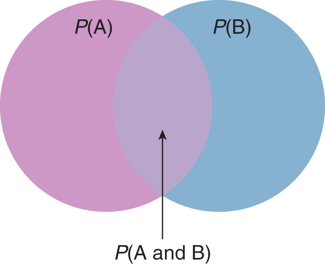
Figure 12.4. Probability of Two Independent Events Co-Occurring **P(A and B) =P(A) ×P(B)
The probability of at least one of two events occurring is equal to the sum of their initial probabilities, minus the probability that they will both occur.
P(A ∪ B) = P(A or B) = P(A) + P(B) − P(A and B)
Equation 12.7
KEY CONCEPT
In probability, when using the word:
- and—multiply the probabilities
- or—add the probabilities (and subtract the probability of both happening together)
Example: In a certain population, 10% of the population has diabetes and 30% is obese. If 7% of the population has both diabetes and obesity, are these events independent? If one chose an individual at random from this population, what would be the probability of that patient having at least one of the two conditions?
Solution: With the numbers given, these events cannot be independent. For independent events, P(A and B) = P(A) × P(B) = P(having diabetes) × P(being obese) = 0.1 × 0.3 = 0.03. In this population, the probability of having diabetes and being obese is 0.07.
To determine the probability of the individual having at least one of the conditions, we use the “or” equation:
P(A or B) = P(A) + P(B) − P(A and B) = 0.1 + 0.3 − 0.07 = 0.33 or 33%
MCAT CONCEPT CHECK 12.4
Before you move on, assess your understanding of the material with these questions.
- Assume the likelihood of having a male child is equal to the likelihood of having a female child. In a series of ten live births, the probability of having at least one male child is equal to:
_________________________________
- Define the following terms:
- Independence:
_________________________________
- Mutual exclusivity:
_________________________________
- Exhaustiveness:
_________________________________
12.5 Statistical Testing
LEARNING OBJECTIVES
After Chapter 12.5, you will be able to:
- Distinguish between hypothesis tests and confidence intervals
- Recall how p-values are calculated during a hypothesis test
- Predict the outcome of a test given its p- and α- values
- Explain the importance of power in statistical testing
Hypothesis testing and confidence intervals allow us to draw conclusions about populations based on our sample data. Both are interpreted in the context of probabilities, and what we deem to be an acceptable risk of error.
Hypothesis Testing
Hypothesis testing begins with an idea about what may be different between two populations. We have a null hypothesis, which is always a hypothesis of equivalence. In other words, the null hypothesis says that two populations are equal, or that a single population can be described by a parameter equal to a given value. The alternative hypothesis may be nondirectional (that the populations are not equal) or directional (for example, that the mean of population A is greater than the mean of population B).
The most common hypothesis tests are z- or t-tests, which rely on the standard distribution or the closely related t-distribution. From the data collected, a test statistic is calculated and compared to a table to determine the likelihood that that statistic was obtained by random chance (under the assumption that our null hypothesis is true). This is our p-value. We then compare our p-value to a significance level (α); 0.05 is commonly used. If the p-value is greater than α, then we fail to reject the null hypothesis, which means that there is not a statistically significant difference between the two populations. If the p-value is less than α, then we reject the null hypothesis and state that there is a statistically significant difference between the two groups. Again, when the null hypothesis is rejected, we state that our results are statistically significant.
The value of α is the level of risk that we are willing to accept for incorrectly rejecting the null hypothesis. This is also called a type I error. In other words, a type I error is the likelihood that we report a difference between two populations when one does not actually exist. A type II error occurs when we incorrectly fail to reject the null hypothesis. In other words, a type II error is the likelihood that we report no difference between two populations when one actually exists. The probability of a type II error is sometimes symbolized by β. The probability of correctly rejecting a false null hypothesis (reporting a difference between two populations when one actually exists) is referred to as power, and is equal to 1 − β. Finally, the probability of correctly failing to reject a true null hypothesis (reporting no difference between two populations when one does not exist) is referred to as confidence. These conditions are summarized in Table 12.1.
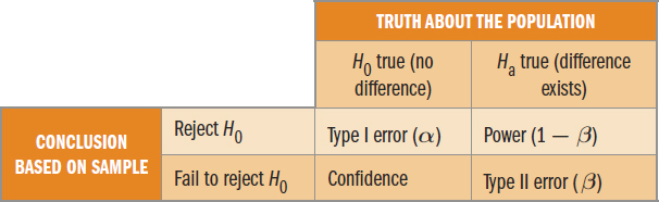
Table 12.1 Results of Hypothesis Testing
Confidence Intervals
Confidence intervals are essentially the reverse of hypothesis testing. With a confidence interval, we determine a range of values from the sample mean and standard deviation. Rather than finding a p-value, we begin with a desired confidence level (95% is standard) and use a table to find its corresponding z- or t-score. When we multiply the z- or t-score by the standard deviation, and then add and subtract this number from the mean, we create a range of values. For example, consider a population for which we wish to know the mean age. We draw a sample from that population and find that the mean of the sample is 30, with a standard deviation of 3. If we wish to have 95% confidence, the corresponding z-score (which would be provided on Test Day) is 1.96. Thus, the range is 30 − (3)(1.96) to 30 + (3)(1.96) = 24.12 to 35.88. We can then report that we are 95% confident that the true mean age of the population from which this sample is drawn is between 24.12 and 35.88.
MCAT CONCEPT CHECK 12.5
Before you move on, assess your understanding of the material with these questions.
- How do hypothesis tests and confidence intervals differ?
- Hypothesis tests:
_________________________________
- Confidence intervals:
_________________________________
- If the p-value is greater than α in a given statistical test, what is the outcome of the test?
_________________________________
- How is the p-value calculated during a hypothesis test?
_________________________________
_________________________________
- True or False: Power is the probability of correctly rejecting the null hypothesis.
12.6 Charts, Graphs, and Tables
LEARNING OBJECTIVES
After Chapter 12.6, you will be able to:
- Recognize when data relationships call for transformation into semilog or log-log plots
- Recall the pros and cons of different types of visual data representation, including pie charts, bar graphs, box plots, maps, graphs, and tables
- Distinguish between exponential and parabolic curves
Because your career will be filled with evidence-based medicine, it is important to be able to recognize and interpret data in multiple forms. We have already considered the mathematical side of statistics; now, let’s take a look at the visual side. On the MCAT, anticipate that most passages in the sciences will be accompanied by a visual aid in some way—frequently, this will be a chart, graph, or data table.
Types of Charts
Charts present information in a visual format and are frequently used for categorical data.
Pie or Circle Charts
Pie or circle charts are used to represent relative amounts of entities and are especially popular in demographics. They may be labeled with raw numerical values or with percent values. The primary downside to pie charts is that as the number of represented categories increases, the visual representation loses impact and becomes confusing. For example, in Figure 12.5, the population of each of the 50 United States and the District of Columbia is presented on a pie chart, but the large number of entities makes the graph incoherent.
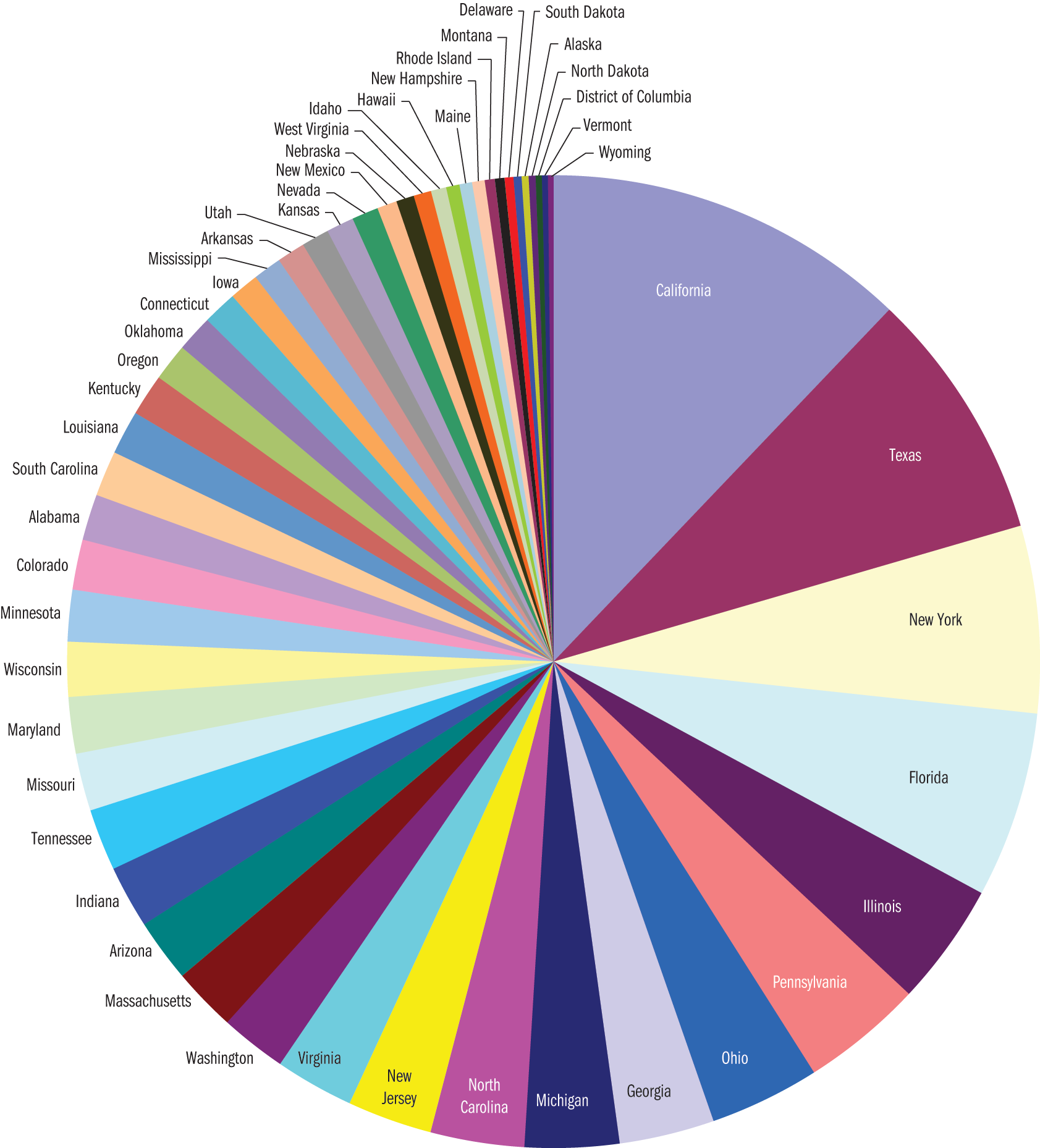
Figure 12.5. Pie Chart of United States Population by State, 2010 Census Pie charts become difficult to interpret when too many categories are included.
MCAT EXPERTISE
Questions about pie charts are likely to be qualitative, asking for the smallest or largest group, or the percentage occupied by one or more groups combined. These questions are unlikely to require additional analysis because pie charts are not dense with information.
BRIDGE
Pie charts are frequently used to present demographic information. Demographics is the statistical arm of sociology and is discussed in Chapter 11 of MCAT Behavioral Sciences Review.
Bar Charts and Histograms
Bar charts and histograms are likely to contain significantly more information than a pie chart for the same amount of page space. Bar charts are used for categorical data, which sort data points based on predetermined categories. The bars may then be sorted by increasing or decreasing bar length. The length of a bar is generally proportional to the value it represents. Wherever possible, breaks should be avoided in the chart because of the potential to distort scale. To that end, be wary of graphs that contain breaks; they may be enlarging the difference between bars. Figure 12.6 shows a representative bar graph for causes of cancer death in the United Statesh in the United States in 2010.
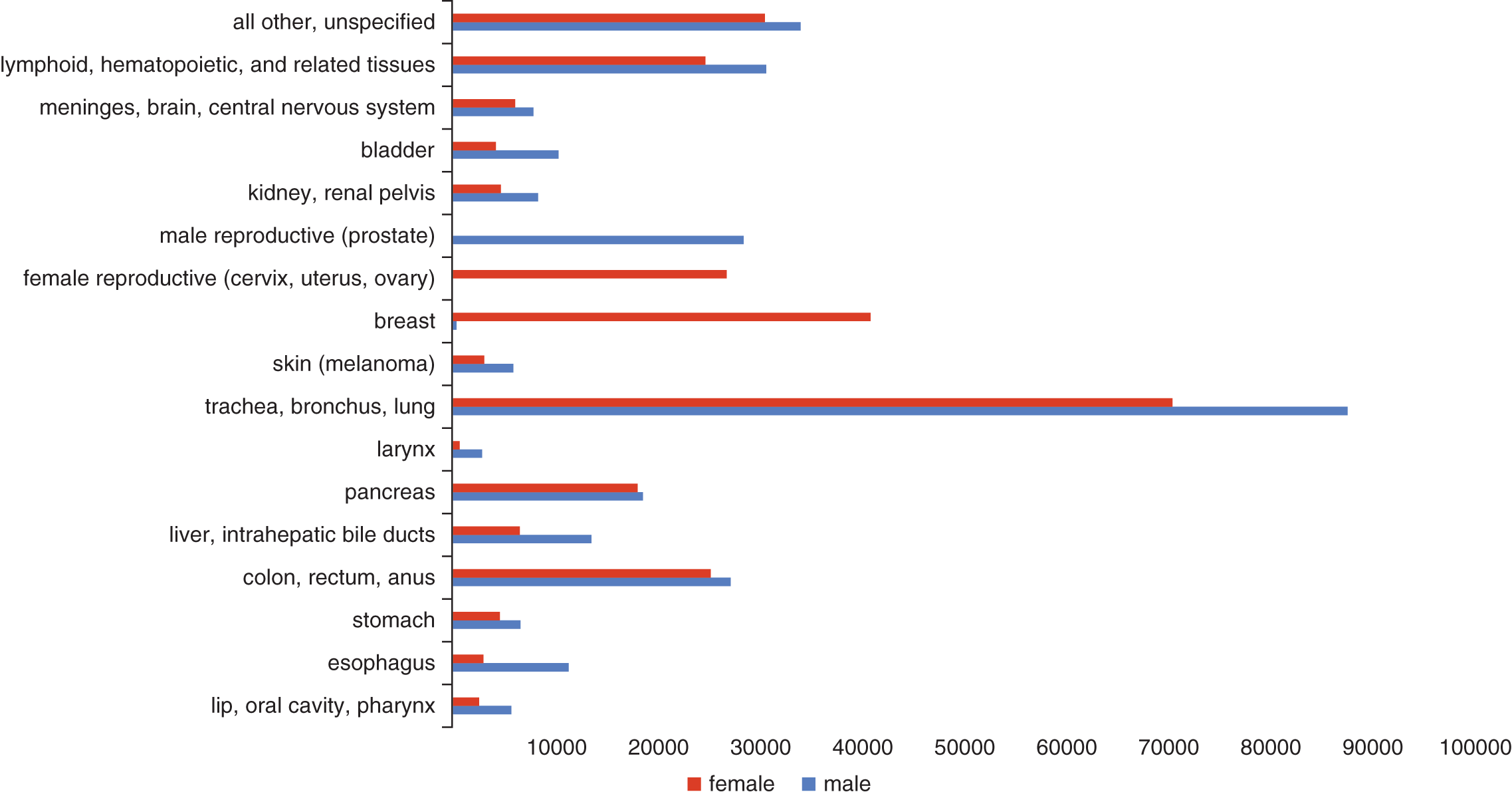
Figure 12.6. Causes of Cancer Death by Type, 2010 Source: Centers for Disease Control and Prevention National Vital Statistics Reports
Histograms present numerical data rather than discrete categories. Histograms are particularly useful for determining the mode of a data set because they are used to display the distribution of a data set.
Box plots are used to show the range, median, quartiles and outliers for a set of data. A labeled box plot, also called a box-and-whisker, is shown in Figure 12.7.
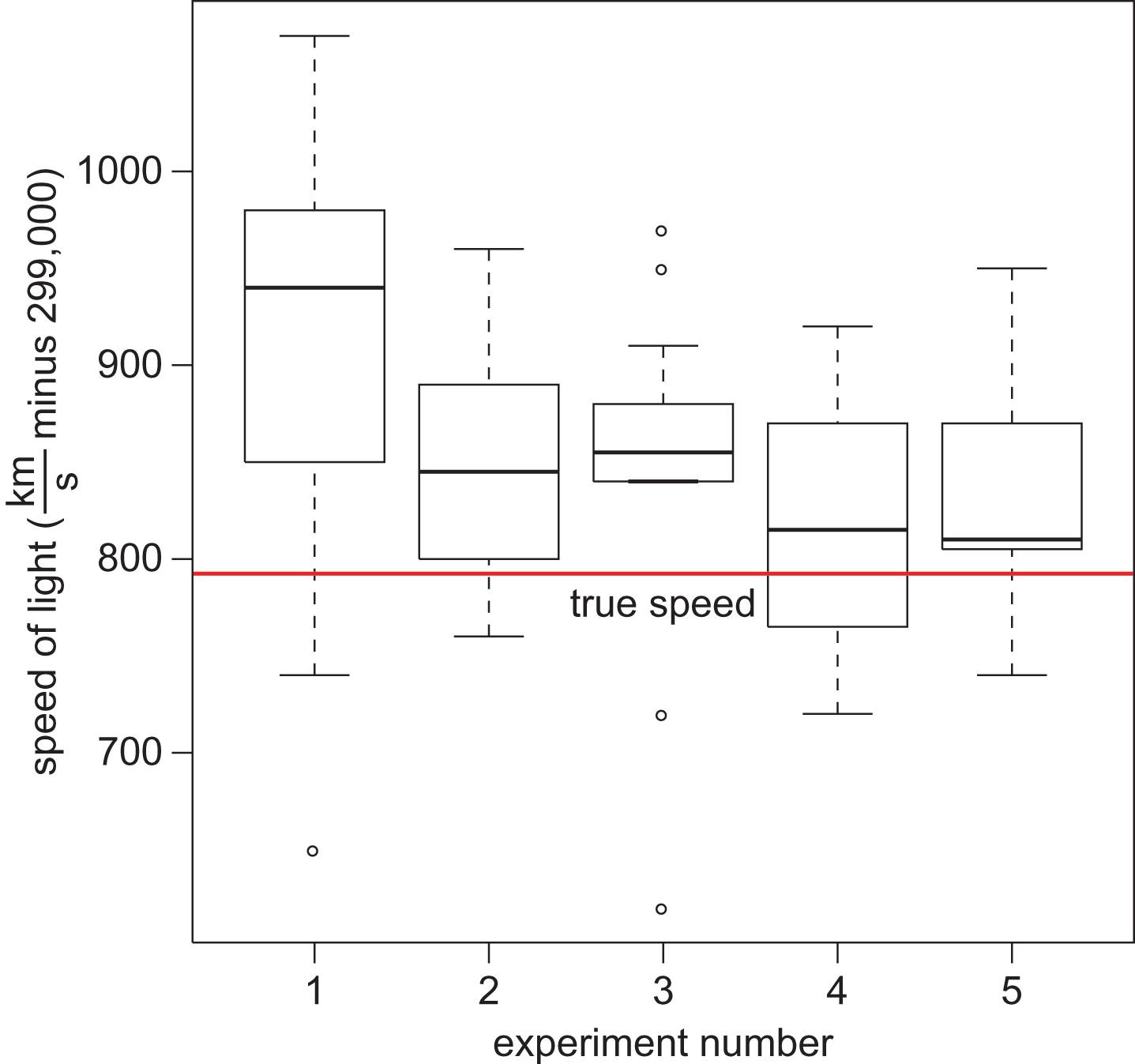
Figure 12.7. Box Plot of Measurements of the Speed of Light
The box of a box-and-whisker plot is bounded by Q1 and Q3; Q2 (the median) is the line in the middle of the box. The ends of the whiskers correspond to maximum and minimum values of the data set. Alternatively, outliers can be presented as individual points, with the ends of the whiskers corresponding to the largest and smallest values in the data set that are still within 1.5 × IQR of the median. Box-and-whisker plots are especially useful for comparing data because they contain a large amount of data in a small amount of space, and multiple plots can be oriented on a single axis.
Maps
In addition to the other forms of charts, data can be illustrated geographically. Maps of health conditions, population density, political districts, and ethnicity are relatively easy to comprehend and may show geographic clustering for some data. The best map data will examine one or at most two pieces of information simultaneously. Any further data may inhibit clarity. A map of population density in each country of the world is shown in Figure 12.8.
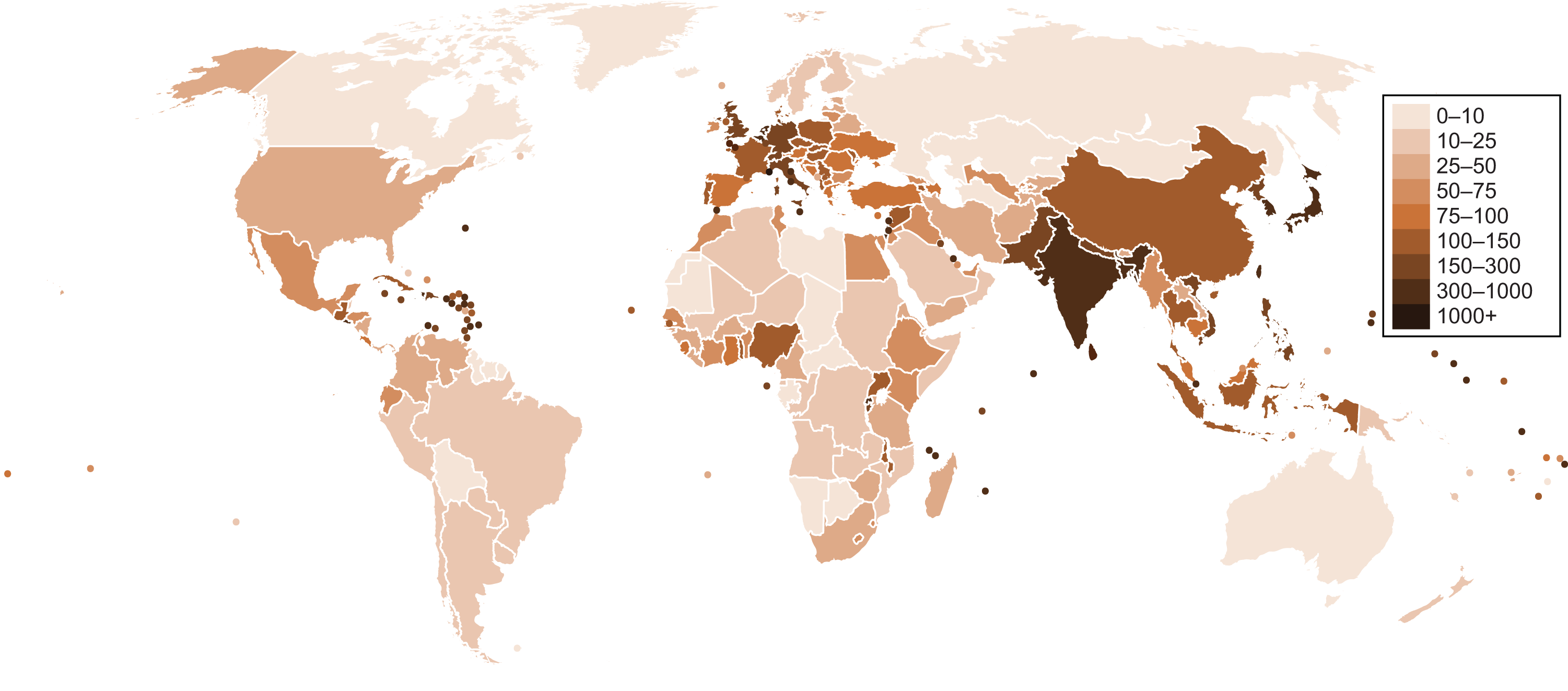
Figure 12.8. Population Density by Country, 2006
Graphs and Axes
While we’re all familiar with constructing graphs—especially scatter plots and line graphs—it is important to know some important features and potential stumbling blocks of graphs as we move toward Test Day. When presented with a graph, you should attempt to draw rough conclusions immediately but should not spend time analyzing all of the details of the graph unless asked to do so by a question. The first thing to do when you encounter a graph on Test Day is to look at the axes.
Linear Graphs
Linear graphs show the relationships between two variables. They generally involve two direct measurements and, strictly speaking, do not have to be a straight line. The shape of the curve on this type of graph may be linear, parabolic, exponential, or logarithmic. These are shown in Figure 12.9. On Test Day, you should be able to recognize at least these four shapes of graphs.
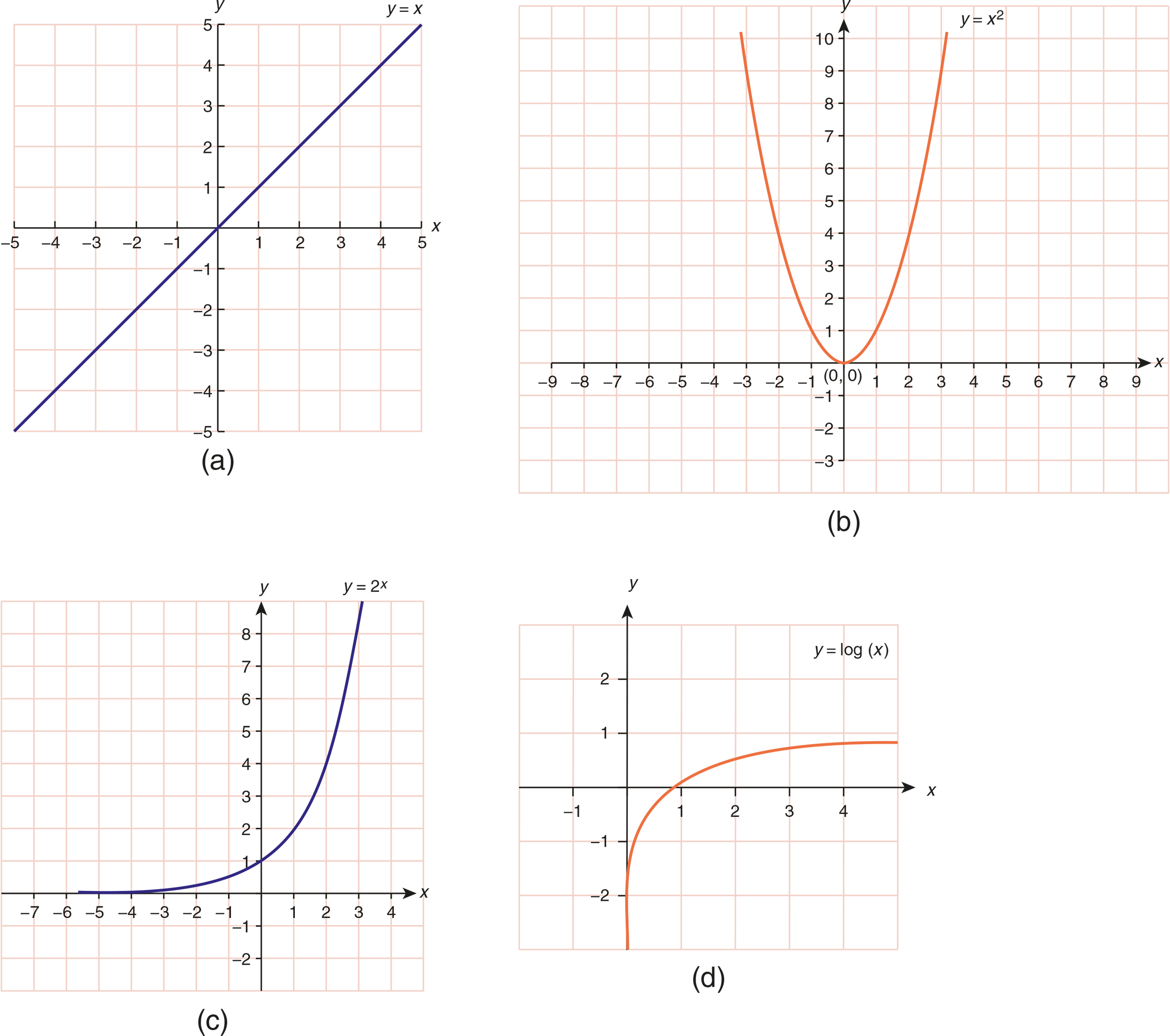
Figure 12.9. Shapes of Common Relationships on a Linear Graph (a) Linear; (b) Parabolic; (c) Exponential; (d) Logarithmic
The axes of a linear graph will be consistent in the sense that each unit will occupy the same amount of space (the distance from 1 to 2 to 3 to 4 on each axis remains the same size). As with bar graphs, be wary of scale and breaks in axes. Where both the shape of the graph and the graph type are linear, we should be able to calculate the slope of the line. Slope (m) is the change in the y-direction divided by the change in the x-direction for any two points:
m=riserun=ΔyΔx
Equation 12.8
MNEMONIC
Slope is like waking up in the morning: Slope is always rise (vertical) over run (horizontal) because you have to get up from bed (rise) before you get moving (run).
Example: Calculate the slope of the line in the graph shown below.
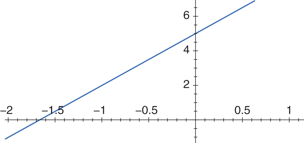
Solution: The slope of a line is equal to the difference in the values of two points in the y-direction divided by the difference in the values of the same two points in the x-direction. The x- and y-intercepts are generally good choices because one of the values will be zero for each point:
m=y2−y1x2−x1=0−5−1.66−0=−5−1.66=553=3
Semilog and Log–Log Graphs
Semilog graphs are a specialized representation of a logarithmic data set. They can be easier to interpret because the otherwise curved nature of the logarithmic data is made linear by a change in the axis ratio. In semilog graphs, one axis (usually the x-axis) maintains the traditional unit spacing. The other axis assigns spacing based on a ratio, usually 10, 100, 1000, and so on. The multiples may be of any number as long as there is consistency in the ratio from one point on the axis to the next. Figure 12.10 shows an example of a semilog plot.
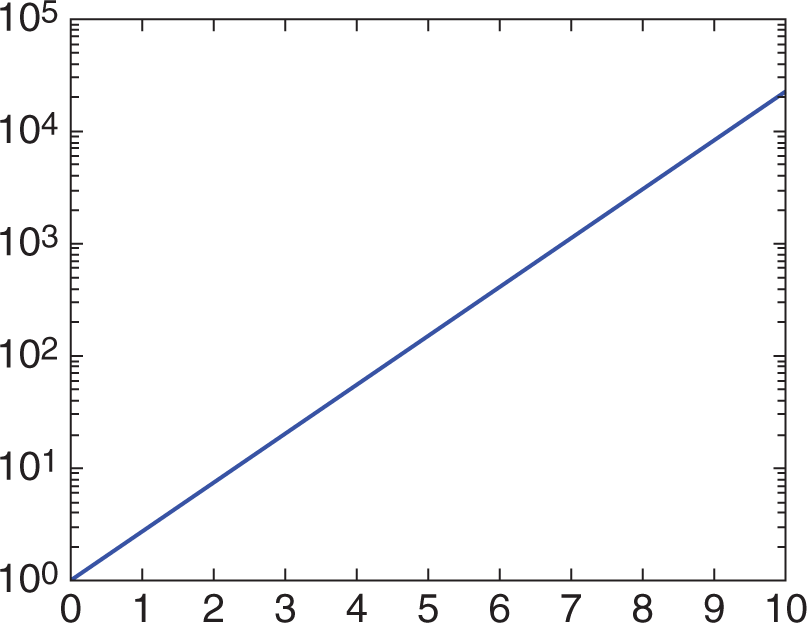
Figure 12.10. A Semilog Plot
KEY CONCEPT
The axes on a graph will determine which type of plot is being used, and provide key information about the underlying relationship between the relevant variables.
In some cases, both axes can be given a different axis ratio to create a linear plot. When both axes use a constant ratio from point to point on the axis, this is termed a log–log graph. Note that the difference between these three plot types (linear, semilog, and log–log) is based on the labeling of the axes. Therefore, it is crucial to pay attention to the axes on Test Day to be able to interpret a graph correctly.
Example: Patients that undergo a positron emission tomography (PET) scan are injected with radioactive Flouride-18 (F-18). The graph below shows the percent of F-18 remaining as a function of time. Typical doses of F-18 are measured in units of becquerels (Bq). If a syringe of F-18 initially contains 0.37 GBq of F-18, approximately how much F-18 is in the syringe after one hour?
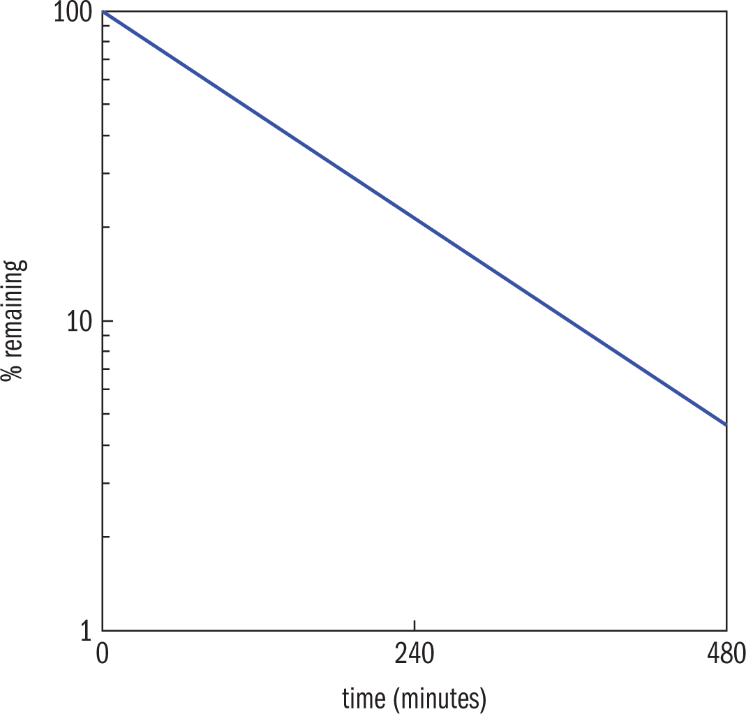
Solution: Notice that the values on theNotice that the values on the y-axis are equally spaced and multiples of ten. That means the y-axis is logarithmic. The x-axis is linear so the graph is a semilog plot. Use the graph to determine the percent remaining, which can then be used to determine the amount remaining.
Start by finding one hour (the known value) on the x-axis. It is one-fourth of the distance between 0 and 240 minutes. Find the corresponding point on the line and then note the location on the y-axis. Between each y-axis label (1, 10, and 100) the axis is divided equally in value, although the marks are unequally spaced. So the eight axis markers between 10 and 100 represent 20, 30, 40, 50, 60, 70, 80, and 90. The point at one hour corresponds to about the third mark below 100, or 70%.
To find the amount of F-18 remaining, the original amount must be multiplied by 0.70. Therefore the correct answer is approximately 0.26 GBq.
Interpreting Tables
Unlike with graphs, you should only take a brief moment to glance at the title of a table before approaching Test Day questions. Tables are more likely to contain disjointed information than either charts or graphs because they often contain categorical data or experimental results. Tables that do not have unusual data values (zeroes, outliers, changes in a trend, and so on) should be approached especially briefly.
When a table does contain significant organization (for example, listing results progressively), this structure is likely to be relevant while answering questions. For example, a trend that suddenly appears or disappears will often require an explanation.
Additionally, when provided with data in the form of a table, you should be able to convert it to a rough graph or to a linear equation. The MCAT may test on the interpretation of slope without actually providing a graph.
MCAT CONCEPT CHECK 12.6
Before you move on, assess your understanding of the material with these questions.
- What type of data relationship is least likely to require transformation into a semilog or log–log plot?
_________________________________
- Fill in the following table with the pros and cons of each type of visual data representation:
Type of Visual Aid Pros Cons Pie Chart Bar Graph Box Plot Map Graph Table
- How do exponential and parabolic curves differ in shape?
- Exponential:
_________________________________
- Parabolic:
_________________________________
12.7 Applying Data
LEARNING OBJECTIVES
After Chapter 12.7, you will be able to:
- Distinguish between correlation and causation
- Relate the statistical results of a study to the impact of those findings on scientific knowledge and policy change
Finally, we have reached the discussion section of an academic paper, in which the data that we have gathered and interpreted is applied to the original problem. We can then begin drawing conclusions and creating new questions based on our results. Because much of this was covered in the discussion on experimental methods in Chapter 11 of MCAT Physics and Math Review, we will be terse in our review here.
Correlation and Causation
As discussed previously, we must be careful with our wording when discussing variable relationships. Correlation refers to a connection—direct relationship, inverse relationship, or otherwise—between data. If two variables trend together, that is as one increases so does the other, there is a positive correlation. If two variables trend in opposite directions (one increases as the other decreases) there is a negative correlation. These relationships can be quantified with a correlation coefficient, a number between –1 and +1 that represents the strength of the relationship. A correlation coefficient of +1 indicates a strong positive relationship, a value of –1 indicates a strong negative relationship, and a value of zero indicates no apparent relationship.
Correlation does not necessarily imply causation; we must avoid this assumption when there is insufficient evidence to draw such a conclusion. If an experiment cannot be performed, we must rely on Hill’s criteria, discussed in Chapter 11 of MCAT Physics and Math Review. Remember that the only one of Hill’s criteria that is uniformly necessary for causation is temporality.
In the Context of Scientific Knowledge
When interpreting data, it is important that we not only state the apparent relationships between data, but also begin to draw connections to other concepts in science and to our background knowledge. At a minimum, the impact of the new data on the existing hypothesis must be considered, although ideally the new data would be integrated into all future investigations on the topic. Additionally, we must develop a plausible rationale for the results. Finally, we must make decisions about our data’s impact on the real world, and determine whether or not our evidence is substantial and impactful enough to necessitate changes in understanding or policy.
Example: A textbook publisher wanted to study the effectiveness of a new Advanced Placement (AP) study aid. From 2006 to 2015 the researchers recruited high schools across the country to participate, and randomly assigned each school to a group—those who received the study aid (Group A) and those who did not (Group B). Grades were tracked in AP Statistics over a 10 year time period. On which three years was there a statistically significant difference between the two groups, and a high likelihood of passing for those who used the study aid?
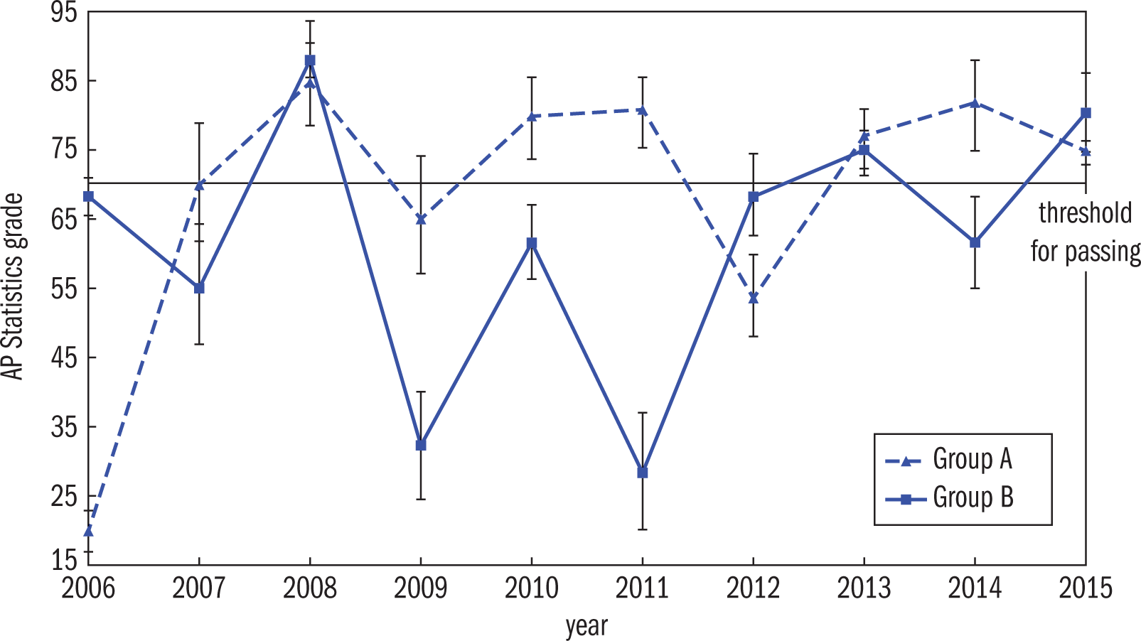
Average AP Grades By Group Error bars show the 95% CI
Solution: In order to support the claim that the study aid helps students pass the AP exam, the evidence should show a statistically significant difference between those who received the aid and those who did not. Further, the true score (which should be within the confidence interval 95% of the time) of those who received the aid should be above passing and the true score of those who did not should be below passing. The data from 2010, 2011, and 2014 fit the description and provide the best support.
MCAT CONCEPT CHECK 12.7
Before you move on, assess your understanding of the material with these questions.
- True or False: Statistical significance is sufficient criteria to enact policy change.
- True or False: Two variables that are causally related will also be correlated with each other.
Conclusion
Congratulations on completing MCAT Physics and Math Review! While it has been a challenging journey, you are now equipped with all of the physics content knowledge and Scientific Inquiry and Reasoning Skills (SIRS) you need to perform well on Test Day. We completed our discussion of the MCAT SIRS by covering the transformation of raw data to actionable information. When taking the MCAT, these concepts may present themselves as the opportunity to use statistical methods and interpretation to draw conclusions, as well as the analysis of figures used as adjuncts to passages and discrete questions. We also briefly reviewed the connections between the real world and research by determining when and how our newfound data can be applied. Ultimately, this will be your role as a physician: constructing a foundation of content knowledge, seeking out new research, and drawing conclusions from that research to improve your patients’ lives and well-being. Good luck as you continue preparing for your MCAT—and your future as an excellent physician.
GO ONLINE
You’ve reviewed the content, now test your knowledge and critical thinking skills by completing a test-like passage set in your online resources!
CONCEPT SUMMARY
Measures of Central Tendency
- Measures of central tendency provide a single value representation for the middle of a group of data.
- The arithmetic mean or average is a measure of central tendency that equally weighs all values; it is most affected by outliers.
- The median is the value that lies in the middle of the data set. Fifty percent of data points are above and below the median.
- The mode is the data point that appears most often; there may be multiple (or zero) modes in a data set.
Distributions
- Distributions have characteristic features that are exemplified by their shape. Distributions can be classified by measures of central tendency and measures of distribution.
- The normal distribution is symmetrical. The mean, median, and mode are all the same in the normal distribution.
- The standard distribution is a normal distribution with a mean of zero and a standard deviation of one; it is used for most calculations.
- 68% of data points occur within one standard deviation of the mean, 95% within two, and 99% within three.
- Skewed distributions have differences in their mean, median, and mode; the skew direction is the direction of the tail of the distribution.
- Bimodal distributions have multiple peaks, although not necessarily multiple modes, strictly speaking. It may be useful to perform data analysis on the two groups separately.
Measures of Distribution
- Range is the difference between the largest and smallest values in a data set.
- Interquartile range is the difference between the value of the third quartile and first quartile; interquartile range can be used to determine outliers.
- Standard deviation is a measurement of variability about the mean; standard deviation can also be used to determine outliers.
- Outliers may be a result of true population variability, measurement error, or a non normal distribution.
- Procedures for handling outliers should be formulated before the beginning of a study.
Probability
- The probability of independent events does not change based on the outcomes of other events.
- The probability of a dependent event changes depending on the outcomes of other events.
- Mutually exclusive outcomes cannot occur simultaneously.
- When a set of outcomes is exhaustive, there are no other possible outcomes.
Statistical Testing
- Hypothesis tests use a known distribution to determine whether a hypothesis of no difference (the null hypothesis) can be rejected.
- Whether or not a finding is statistically significant is determined by the comparison of a p-value to the selected significance level (α). A significance level of 0.05 is commonly used.
- Confidence intervals are a range of values about a sample mean that are used to estimate the population mean. A wider interval is associated with a higher confidence level (95% is common).
Charts, Graphs, and Tables
- Pie charts (circle charts) and bar charts are both used to compare categorical data.
- Histograms and box plots (box-and-whisker plots) are both used to compare numerical data.
- Maps are used to compare up to two demographic indicators.
- Linear, semilog, and log–log plots can be distinguished by their axes.
- Slope can be calculated most easily from linear plots.
- Tables may contain related or unrelated categorical data.
Applying Data
- Correlation and causation are separate concepts that are linked by Hill’s criteria.
- Data must be interpreted in the context of the current hypothesis and existing scientific knowledge.
- Statistical and practical significance are distinct.
ANSWERS TO CONCEPT CHECKS
**12.1**
- The mean is the best measure of central tendency for a data set with a relatively normal distribution. The mean performs poorly in data sets with outliers.
Median: The fifth position of 2, 4, 4, 6, 9, 21, 23, 23, 25 is 9 Mode: There are two numbers that each appear twice: 4 and 23. These are both modes of this data set.
- Mean:25+23+23+6+9+21+4+4+29=1179=13
**12.2**
- The mean of a right (positively) skewed distribution is to the right of the median, which is to the right of the mode.
- Any distribution can be mathematically or procedurally transformed to follow a normal distribution by virtue of the central limit theorem, which is beyond the scope of the MCAT. Regardless, a distribution that is not normal may still be analyzed with these measures.
- Bimodal distributions have two peaks, whereas normal or skewed distributions have only one.
**12.3**
- Outliers can be defined as data points more than 1.5 × IQR below Q1 or above Q3. They can also be defined as data points more than 3σ above or below the mean. The cutoff values calculated through the two methods are likely to be different, and the selection of one method over the other is one of preference and study design. In general, the use of the standard deviation method is superior.
- Where the data are not available, the range can be approximated as four times the standard deviation. For this data set, the relationship fails. The range is 9, which is only a little more than twice the standard deviation. This is because the data set does not fall in a normal distribution.
- The average distance from the mean will always be zero. This is why, in calculations of standard deviation, we always square the distance from the mean and then take the square root at the end—it forces all of the values to be positive numbers, which will not cancel out to zero.
**12.4**
- Simplify this question by rewording it as the probability of not having all female children. Having at least one male child and having all female children are mutually exclusive events, and no other possibilities can occur. Thus, the probability of having all female children is (0.5)10 and the probability of having at least one male child is 1 – (0.5)10, or 99.90%.
- Independence is a condition of events wherein the outcome of one event has no effect on the outcome of the other. Mutual exclusivity is a condition wherein two outcomes cannot occur simultaneously. When a set of outcomes is exhaustive, there are no other possible outcomes.
**12.5**
- Hypothesis tests are used to validate or invalidate a claim that two populations are different, or that one population differs from a given parameter. In a hypothesis test, we calculate a p-value and compare it to a chosen significance level (α) to conclude if an observed difference between two populations (or between a population and the parameter) is significant or not. Confidence intervals are used to determine a potential range of values for the true mean of a population.
- If the p-value is greater than α, then we fail to reject the null hypothesis.
- After the test statistic is calculated, a computer program or table is consulted to determine the p-value of the statistic.
- True. Power is the probability that the individual rejects the null hypothesis when the alternative hypothesis is true for the population.
**12.6**
- Linear relationships can be analyzed without any data or axis transformation into semilog or log–log plots.
-
Type of Visual Aid Pros Cons Pie Chart Easily constructed; useful for categorical data with a small number of categories. Easily overwhelmed with multiple categories. Difficult to estimate values with circles.
Bar Graph Multiple organization strategies. Good for large categorical data sets. Axes are often misleading because of sizeable breaks.
Box Plot Information-dense; can be useful for comparison. May not highlight outliers or mean value of a data set. Only useful for numerical data.
Map Provide relevant and integrated geographic and demographic information. May only be used to represent at most two variables coherently.
Graph Provide information about relationships. Useful for estimation. Axis labels and logarithmic scales require careful interpretation.
Table Categorical data can be presented without comparison. Does not require estimation for calculations. Disorganized or unrelated data may be presented together.
- Exponential and parabolic curves both have a steep component; however, exponential curves have horizontal asymptotes and become flat on one side while parabolic curves are symmetrical and have steep components on both sides of a center point.
**12.7**
- False. As discussed in the last chapter, there must be practical (clinical) as well as statistical significance for a conclusion to be useful.
- True. While two variables that are correlated are not necessarily causally related, all variables that are causally related must be correlated in some way (direct relationship, inverse relationship, or otherwise).
SCIENCE MASTERY ASSESSMENT EXPLANATIONS
1. C
The mean is computed by taking the sum of all of the data points and dividing by the total number of data points. If a very large data point was included, the sum would be significantly larger, inflating the mean. This observation justifies (C). On the other hand, since the median is the middle number and the mode is the most common value, the inclusion of outliers would have minimal effect on these measures.
2. B
The mean is to the left of the median, which implies that the tail of the distribution is on the left side; therefore, this distribution is skewed left. It would be expected that there would be a low plateau on the left side of the distribution, which accounts for the shift in the mean.
3. B
The median is the central data point in an ordered list. Because this data set has seven numbers, the central point will be in the fourth position. Reordered, the list reads: 2, 4, 4, 7, 17, 23, 53. Thus, the median is 7. (A), 4, is the mode while (C), 15.7, is the mean.
4. B
Based on the population description in the question stem, we would expect to see a large number of finches with small beaks, a very small number of finches with intermediate beaks, and a large number of finches with large beaks. This pattern is consistent with a bimodal distribution, choice (B).
5. B
Approximately 95% of values fall within two standard deviations (±2σ) of the mean for a normal distribution. A confidence interval is constructed using the same values. Approximately 68% of the values are within one standard deviation, and 99% are within three standard deviations, eliminating the other answer choices.
6. C
When two events are independent of each other, the probability of them occurring simultaneously is equal to the product of the probability of each occurring separately. Thus, for weekly fast food consumption and prevalence of cardiovascular disease to be independent, the probability of both occurring must be (20%)(48%) = 9.6%, supporting (C). While (D) is a tempting answer choice, a lack of cardiovascular disease among people who eat fast food would not imply independence of these factors, rather it would imply that fast food consumption actually decreases or eliminates the likelihood of cardiovascular disease.
7. A
Because the error is in data transfer, the original source of data can be consulted to allow for the inclusion of the correct data point. An error in instrument calibration may introduce bias; while this should not affect the standard deviation of a sample, it would certainly affect the mean. The instrument would have to be recalibrated, and the relevant data points would have to be measured again to correct for this type of outlier, eliminating choice (B). A skewed distribution is one that has a long tail. In this case, it may be more challenging to determine if a particular value is an outlier or simply a value in the long tail of the distribution. Repeated sampling or a large sample size is usually required to determine if a sample is truly skewed, eliminating choice (C). An anomalous result is challenging to interpret, and how to correct for the result may be unclear. In some cases, the result should be inflated or weighted more heavily to reflect its significance; in other cases, it should be interpreted as a regular value. In still other cases, it is appropriate to drop the anomalous result. This decision should ideally be made before the study even begins, but this still certainly requires more consideration than simply checking a result from one’s original data set, eliminating choice (D) and making choice (A) correct.
8. A
Because one parent is homozygous for both traits, we are only concerned with the other parent. This parent has a 50% chance of transmitting each independent trait, and thus a 25% chance of transmitting both (12×12=14). This probability is the same for both pregnancies because they are independent events; thus, the probability that both children exhibit both traits is: 14×14=116=0.0625=6.25%.
9. C
With data about percentages, we can only draw conclusions about percentages. Thus any information about number of people, as in (A), is incorrect. This map shows us that a higher percentage of the residents in the middle of the country are over 65 in comparison to other parts of the country. There are, of course, exceptions to this rule, including Florida, the Pacific Coast, and parts of Appalachia, which are all in the top category. Even so, there appears to be a clustering of counties with a high percentage of individuals over 65 in the middle of the country. We also cannot say that most of the population is over 65 in any place on this map because we are not given actual values for the percentages. There may be a plurality, but there is insufficient information to posit a majority, eliminating (B). The map gives no indication of migration patterns, so we can also eliminate (D).
10. A
To increase the confidence level, one must increase the size of the confidence interval to make it more likely that the true value of the mean is within the range. Therefore, the confidence interval must become wider.
11. D
Standard deviation is the most common measure of distribution. It is the most closely linked to the mean of a distribution and can be used to calculate p-values, which are probabilities (specifically, p-values are the probability that an observed difference between two populations is due to chance).
12. C
Outliers can be determined with respect to the interquartile range, Q3-Q1. The interquartile range for this box plot is 2280 - 2075, or 205. Values that are 1.5 times IQR below Q1 or above Q3 are considered outliers. 2075 - 1.5 times 205 is approximately 2075 - 300, or 1775 (actual = 1767.5). Therefore, 1575 is an outlier. 2280 + 1.5 times 205 is approximately 2580 (actual = 2587.5). Therefore, 2600 is also an outlier.
13. D
The attendant hypothesized that glucose in ice cream was the cause of the increase in violent behavior and designed an observational study. While there was an increase in assaults with an increase in ice cream sales, this relationship is a correlation. Correlation does not prove causation. Thus, the conclusion that glucose was the cause is a significant flaw, making (D) the correct answer.
14. D
Because the histogram contains two peaks with a valley in between, it is a bimodal distribution. The color separation of two distinct populations provides evidence that there is a qualitative difference in the data between the two peaks, thus the data should be analyzed according to gender. There is indeed only one mode, at 5’6". This is the measurement with the largest number of corresponding data points.
15. C
When considering whether the findings of a study merit policy change, both the statistical and clinical significance must be evaluated. In comparing the difference in both the systolic and diastolic blood pressure before and after treatment, the effect of the drug is minimal. While the results are statistically significant, it is very unlikely that this small reduction would lead to a significant clinical improvement. Thus, the doctor should not advocate, making (C) the correct answer.
GO ONLINE
Consult your online resources for additional practice.
EQUATIONS TO REMEMBER
(12.1) Arithmetic mean: x¯=∑ i=1nxin
(12.2) Median position: median position=(n+1)2
(12.3) Range: range = xmax − xmin
(12.4) Interquartile range: IQR = Q3 − Q1
(12.5) Standard deviation: σ=∑i=1n(xi−x¯)2n−1
(12.6) Probability of two independent events co-occurring: P(A ∩ B) = P(A and B) = P(A) × P(B)
(12.7) Probability of at least one event occurring: P(A ∪ B) = P(A or B) = P(A) + P(B) − P(A and B)
(12.8) Slope: m=riserun=ΔyΔx
SHARED CONCEPTS
Behavioral Sciences Chapter 11
Social Structure and Demographics
Biology Chapter 12
Genetics and Evolution
General Chemistry Chapter 5
Chemical Kinetics
Physics and Math Chapter 1
Kinematics and Dynamics
Physics and Math Chapter 10
Mathematics
Physics and Math Chapter 11
Reasoning About the Design and Execution of Research