Protein Structure and Function

Introduction

Chapter 3 Protein Structure and Function Computationally designed, hypothetical four-stranded fiber protein viewed down the fiber axis. Using advanced methods for protein design, the amino acid sequence of the

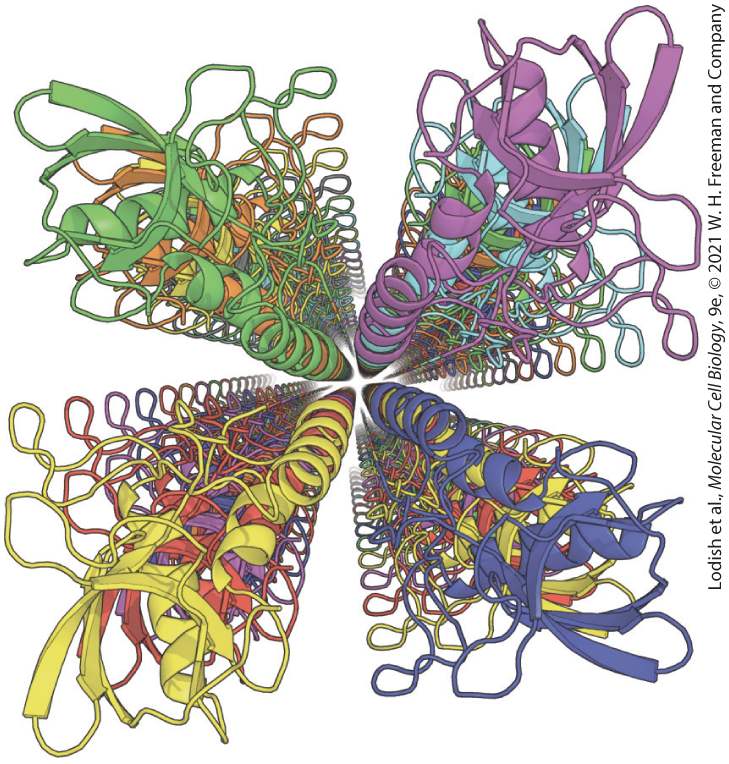
staphylococcal nuclease protein was modified so that the individual, folded protein chains (shown in different colors) would stack into long strands. The design predicts that four long strands would assemble into a four-stranded fiber held together by the binding of hydrophobic helices located in the center of the fiber. [Data from H. Shen et al., 2018, Science 362:705–709.]

3.5 Purifying, Detecting, and Characterizing Proteins

3.6 Proteomics Proteins, which are polymers of amino acids called polypeptides, fold into three-dimensional structures of many sizes and shapes. Their threedimensional diversity principally reflects variations in their amino acid sequences and in the lengths of the polypeptides. In general, a polypeptide will fold into only one or a few closely related three-dimensional shapes — called conformations. A key concept in understanding how a protein works is that its function is often derived from its three-dimensional structure, and its three-dimensional structure is determined by its amino acid sequence and the noncovalent interactions that stabilize its structure. In many cases, the conformation, and thus the function, of a protein can change when that protein associates noncovalently or covalently with other molecules or ions. Through these associations, the function — also called the activity — of a protein can be regulated (e.g., turned “on” or “off,” or “up” or “down”) to permit cells to adapt to changing conditions. Altered conditions include changes in nutrient availability (Chapter 21), hormonal signaling (Chapters 15 and 16), communication with other cells

(Chapters 20 and 23), the developmental state of the organism, and the presence of pathogens (Chapter 24), along with many other factors. How many proteins are there in a typical eukaryotic cell? We can calculate that there are about protein molecules in a mammalian hepatocyte (a liver cell). (This calculation is worked out in Section 3.1.) It is estimated that a hepatocyte contains about 10,000 different proteins; thus each cell, on average, contains close to a million molecules of each type of protein. In reality though, the abundances of different proteins vary widely, from the quite rare insulin-binding receptor protein ( molecules per cell) to the structural protein actin ( molecules per cell). Every cell closely regulates the abundance of each of its proteins so that they are present in the appropriate quantities to support the cell’s needs at any given time. We will learn more about the mechanisms used by cells to regulate protein levels later in this chapter and in Chapters 8 and 9. Because of their many different shapes and chemical properties, proteins can perform a dazzling array of functions inside and outside cells that either are essential for life or provide a selective evolutionary advantage to the cell or organism that contains them. It is, therefore, not surprising that characterizing the structures and activities of proteins — and how these change in response to regulation — is a fundamental prerequisite for understanding how cells work. Much of this textbook is devoted to examining how proteins act with one another or with other types of molecules (e.g., DNA) to allow cells to live and function properly. In this chapter we emphasize the basic principles underlying the structures and

functions of proteins and the regulation of their activity. We also look at some of the many methods used to study them. Although their structures are diverse, most proteins can be grouped into a few broad functional classes. Structural proteins, for example, determine the shapes of cells and their extracellular environments and serve as guide wires or rails to direct the intracellular movement of molecules and organelles. Structural proteins are usually formed by the assembly of multiple protein subunits into very large and often very long structures. Scaffold proteins bring other proteins together into ordered arrays to perform specific functions more efficiently than those proteins would if they were not assembled together. Enzymes are proteins that catalyze chemical reactions (sometimes called molecular transformations). These molecular transformations are the fundamental activities in metabolic pathways (Chapter 12). They can also result in the modification of proteins to alter their activities (e.g., phosphorylation and dephosphorylation to activate and inactivate other proteins). Membrane transport proteins are embedded in cellular membranes and permit the flow of ions and molecules across the membranes. Regulatory proteins act as signals, sensors, and switches to control activities of cells by altering the functions of other proteins and genes. Regulatory proteins include signaling proteins, such as some hormones and cell-surface receptors that transmit extracellular signals to the cell interior. Motor proteins are responsible for the movement of other proteins, organelles, and cells — even whole organisms. There are additional proteins that don’t fit neatly into one of these classes. For example, fish that live in frigid waters — the Antarctic notothenioids and Arctic cods — have antifreeze proteins in

their circulatory systems to prevent water crystallization. Many proteins are members of more than one class, such as some cell-surface signaling receptors that are enzymes and regulatory proteins because they transmit signals from outside to inside cells by catalyzing chemical reactions. To accomplish their diverse missions efficiently, some proteins assemble into very large complexes, often called molecular machines. How do proteins perform so many diverse functions? They do so by exploiting three simple mechanisms. The most fundamental is binding: proteins bind to one another, to other macromolecules such as DNA, and to small molecules and ions. Binding is based on molecular complementarity between a protein and its binding partner, as described in

Chapter 2. A second mechanism is enzymatic catalysis. In enzymes, the proper conformation of the protein will place some amino acid side chains and some carboxyl and amino groups of its backbone into positions that permit the catalysis of covalent bond rearrangements in other molecules (called substrates of the enzyme). A third mechanism is regulation of protein activity. Typically, a protein’s shape or activity is altered through noncovalent (binding) or covalent (catalysis) association of molecules or ions with the protein. In many cases, this binding or catalysis induces a conformational change in the protein and that influences its activity. A complete understanding of how proteins permit cells to live and thrive requires that we identify and characterize all of the proteins used by a cell. In a sense, molecular cell biologists want to compile a complete protein “parts list” and then construct a “user’s manual” that describes how these proteins work. Compiling a comprehensive inventory of proteins has

become feasible in recent years thanks to the sequenced genomes — complete sets of genes — of many organisms. From a computer analysis of a genome’s sequence, researchers can deduce the amino acid sequences and approximate number of different types of proteins the genome encodes (see Chapter 6). It is also possible to determine the sequences and relative amounts of a substantial fraction of the messenger RNAs (mRNAs) in individual cells or most of the mRNAs (the transcriptome) from a collection of similar cells and thus deduce what subset of proteins encoded in the genome is made (expressed) in a given type of cell. DNA and mRNA sequencing are indirect methods of characterizing the potential collection of proteins in cells. There are also methods that directly measure the collection of proteins in samples of cells, which we discuss in Sections 3.5 and 3.6. The term proteome was coined to refer to the entire protein complement of an organism, organ, or a particular type of cell within an organism. The human genome contains about 21,500 genes that encode proteins. However, variations in mRNA production, such as alternative splicing (see

Chapter 9), and more than a hundred types of protein modifications may generate hundreds of thousands of distinct types of human proteins. By comparing the sequences and structures of proteins of unknown function with those of proteins of known function, scientists can often deduce much about what the unknown proteins do. In the past, a protein’s function was characterized by genetic, biochemical, or physiological methods before the particular protein had been identified. In the modern genomic and proteomic era, a protein is often identified before its function is determined.

In this chapter, we begin our study of how the structure of a protein gives rise to its function, a theme that recurs throughout this book (Figure 3-1). In Section 3.1, we examine how linear chains of amino acids are arranged in a three-dimensional structural hierarchy. The next section discusses how proteins fold into these structures. We then turn to protein function, focusing on enzymes, those proteins that catalyze chemical reactions. Our focus on protein structure and function is part of a broader interest in cell biology in the principles relating biological structure and function. These principles were initially formulated by biologists Johann von Goethe (1749–1832), Ernst Haeckel (1834–1919), and D’Arcy Thompson (1860– 1948), whose work has been widely influential in biology and beyond. Indeed, their ideas greatly influenced the school of organic architecture pioneered in the early twentieth century that is epitomized by the dicta “form follows function” (Louis Sullivan) and “form is function” (Frank Lloyd Wright). After considering protein structure and function, we turn to various mechanisms that cells use to control the activities and life spans of proteins. Particularly important control mechanisms are allosteric effector-binding, covalent phosphorylation, and ubiquitinylation of proteins. The chapter concludes with a discussion of commonly used techniques for identifying, isolating, and characterizing proteins, and a discussion of the burgeoning field of proteomics.

FIGURE 3-1 Overview of protein structure and function. (a) Proteins have a hierarchical structure. A polypeptide’s linear sequence of amino acids linked by peptide bonds (primary structure) folds into local helices or sheets (secondary structure) that pack into a complex three-dimensional shape (tertiary structure). Some individual polypeptides associate into multichain complexes (quaternary structure), which in some cases can be very large, consisting of tens to hundreds of subunits (supramolecular complexes). (b) Proteins perform numerous functions, including organizing the genome, organelles, cytoplasm, protein complexes, and membranes in three-dimensional space (structure); monitoring the environment and transmitting information (signaling); moving small molecules and ions across membranes (transport); catalyzing chemical reactions that result in the molecular transformation of one molecule into another; and generating force for movement (via motor proteins). These functions and others arise from mechanisms involving binding, catalysis, and regulation. Description In illustration A, the primary (sequence) structure leads to the secondary (local folding and hydrogen bonding) structure that further leads to tertiary (overall conformation) structure. This leads to a quaternary (multimeric) structure which further leads to a supramolecular (large-scale assembly) structure. In illustration B, the tertiary, quaternary, and supramolecular structures lead to several functions like binding, catalysis, and regulation. These further help in signaling, transport, molecular transformation, movement, and structure.

3.1 Hierarchical Structure of Proteins

3.1 Hierarchical Structure of Proteins Here we consider the architecture of proteins at four levels of organization: primary, secondary, tertiary, and quaternary (Figure 3-2).

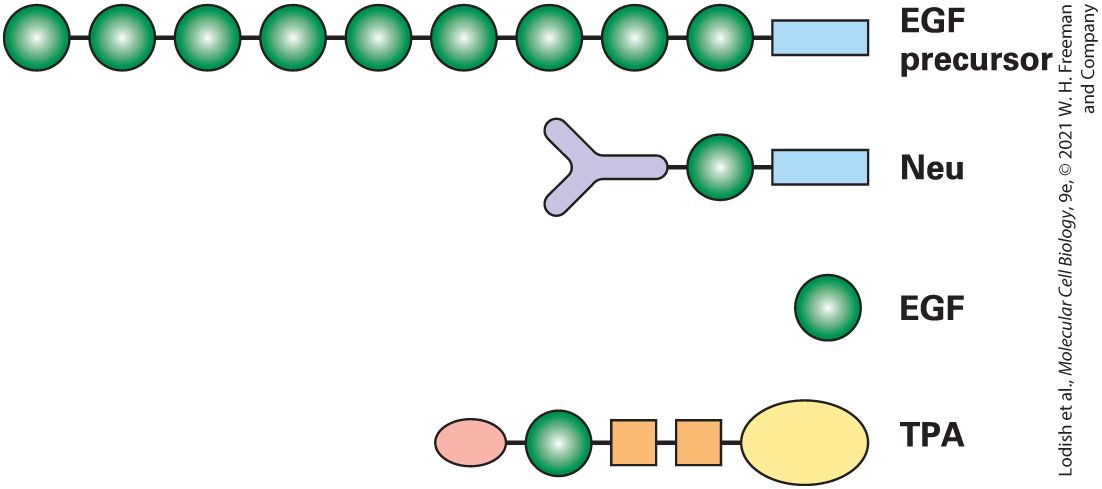
FIGURE 3-2 Four levels of protein hierarchy. (a) The linear sequence of amino acids linked together by peptide bonds is the primary structure. (b) Folding of the polypeptide chain into local α helices or β sheets represents secondary structure. (c) Secondary structural elements, together with various loops and turns in a single polypeptide chain, pack into a larger, independently stable tertiary structure, which may include distinct domains. (d)

The Primary Structure of a Protein Is Its Linear Arrangement of Amino Acids

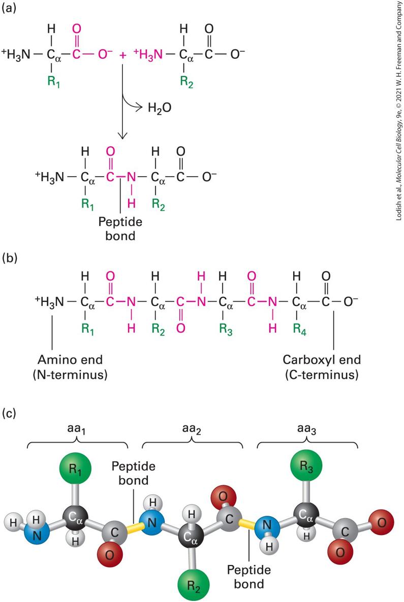
Some proteins consist of more than one polypeptide associated together in a quaternary structure. Description In illustration a, the primary structure shows the sequence of amino acid residues; Ala, Glu, Val, Thr, Asp, Pro, Gly. In illustration b, the secondary structure shows a ribbonlike structure twisted into a spiral-shape alpha-helix and thread-like structure running parallel to each other called beta-sheets. In illustration c, the tertiary structure shows an overall three-dimensional structure of a protein, caused by folding of the whole protein. The structure forms by joining of alpha-helix and beta-sheets, labeled domain. In illustration d, the quaternary structure shows two polypeptide chains. The Primary Structure of a Protein Is Its Linear Arrangement of Amino Acids As discussed in Chapter 2, proteins are polymers constructed out of 20 different types of amino acids. Individual amino acids are linked together in linear chains by covalent amide bonds, called peptide bonds, formed between the carboxyl group of one amino acid and the amino group of the adjacent amino acid (Figure 3-3a). An amino acid in a protein chain is sometimes referred to as a residue. The repeated amide N, α carbon , carbonyl C, and oxygen atoms of each amino acid residue form the backbone of a protein molecule from which the various side-chain groups project (Figure 3-3b, c). Thus one end of a protein has a free (unlinked) amino group (the N-terminus) and the other end has a free carboxyl group (the C-terminus). The primary structure of a protein is simply the linear

covalent arrangement, or sequence, of the amino acid residues that compose it and is conventionally written with its N-terminal amino acid on the left and its C-terminal amino acid on the right. The amino acids are numbered sequentially starting from the N-terminus.

FIGURE 3-3 Structure of a polypeptide. (a) Individual amino acids are linked together by peptide bonds, which form via reactions that result in a loss of water. , , and so on, represent the side chains (R groups) of amino acids. (b) Linear polymers of amino acids linked by peptide bonds are called polypeptides, which have a free (unlinked) amino end (N-terminus) and a free carboxyl end (C-terminus). (c) A ball-and-stick model shows peptide bonds (yellow) linking the amino nitrogen atom (blue) of one amino acid (aa) with the carbonyl carbon atom (gray) of an adjacent one in the chain. The R groups (green) extend from the α-carbon atoms (black) of the amino acids. These side chains largely determine the distinct properties of individual proteins. Description The illustration labeled (a) shows that amino acids are joined together by peptide bonds. The carboxylic end of one amino acid (with R subscript 1 side chain) bonds with the amino end of second amino acid (with R subscript 2 side chain) and results in the loss of a water molecule. The illustration labeled (b) shows a linear polypeptide chain with one end having N H subscript 3 superscript positive and labeled, amino terminal (N-terminus); and opposite end with C doubled O, single bond O superscript negative labeled, carboxyl end (C-terminus). The polypeptide chain has four amino acids linked to one-another by polypeptide bonds. The illustration labeled (c) shows a ball-and-stick model of a linear tripeptide chain. The carboxyl group carbon of amino acid 1 is bonded to the amino group nitrogen of amino acid 2; and the carboxyl group carbon of amino acid 2 is bonded to the amino group nitrogen of amino acid 3. Both bonds are labeled peptide bonds. The first primary structure of a protein determined was that of insulin in the early 1950s. Today the number of known protein sequences exceeds 10 million and is growing daily. Many terms are used to denote the chains formed by the polymerization of amino acids. A short chain of amino acids linked by peptide bonds and having a defined sequence is called an oligopeptide, or simply a peptide; longer chains are referred to as polypeptides. Peptides generally contain fewer than 20–30 amino acid

residues, whereas polypeptides are often 200–500 residues long and can be longer. The longest protein described to date is the muscle protein titin, some forms of which are more than 34,000 residues long. We generally reserve the term protein for a polypeptide (or complex of polypeptides) that has a well-defined three-dimensional structure, although there are exceptions described later in this chapter. The size of a protein or a polypeptide is expressed either as its mass in daltons (a dalton is 1 atomic mass unit) or as its molecular weight (MW), which is a dimensionless number equal to the mass in daltons. For example, a 10,000-MW protein has a mass of 10,000 daltons (Da), or 10 kilodaltons (kDa). In Section 3.5, we will consider different methods for measuring the sizes and other physical characteristics of proteins. The precise molecular weight of a protein that has not been covalently modified is readily determined by summing up the weights of all of its constituent amino acids as determined from its amino acid sequence. The proteins encoded by the yeast genome, for example, have an average molecular weight of 52,728 and contain, on average, 466–amino acid residues. The average molecular weight of amino acids in proteins is 113, taking into account their average relative abundances. This value can be used to estimate the number of residues in a protein of unknown sequence if you know its molecular weight or, conversely, to estimate from the number of residues in a protein its likely molecular weight. Covalent modification of one or more amino acids in a protein — for example, by phosphorylation or glycosylation (see Chapters 2 and 13) — alters the mass of those residues and thus the mass of the protein in which they reside.

Secondary Structures Are the Core Elements of Protein Architecture

In the introduction we noted that a eukaryotic cell, on average, contains close to molecules of protein. How do we estimate this? Let’s do a simple calculation for a hepatocyte (a major type of cell in the mammalian liver). A hepatocyte, roughly a cube 15 μm (0.0015 cm) on a side, has a volume of (or milliliters, ml). Assuming a cell density of 1.03 g/ml, the cell would weigh . Since protein accounts for approximately 20 percent of a cell’s weight, the total weight of cellular protein is . Assuming that an average protein has a molecular weight of about 53,000 g/mol, we can calculate the total number of protein molecules per hepatocyte as about from the total protein weight and Avogadro’s number, the number of molecules per mole of any chemical compound . Secondary Structures Are the Core Elements of Protein Architecture The second level in the hierarchy of protein structure is secondary structure. Secondary structures are stable spatial arrangements of segments of a polypeptide chain held together by hydrogen bonds between backbone amide and carbonyl groups and often involving repeating structural patterns. The propensity of a segment of a polypeptide chain to form any given secondary structure depends on its amino acid sequence (see Section 3.2). A single polypeptide may contain multiple types of secondary structure in various portions of the chain, depending on its sequence. The principal secondary structures are the alpha (α) helix, the beta (β) sheet, and the short, U-shaped beta (β) turn. Parts of a

polypeptide that don’t form these secondary structures may nevertheless have a well-defined, stable shape and are said to have an irregular structure. The term random coil applies to highly flexible parts of a polypeptide chain that have no stable, fixed three-dimensional structure. Random coils are said to be disordered. In an average protein, 60 percent of the polypeptide chain exists as α helices and β sheets; the remainder of the molecule is in irregular structures, coils, and turns or is disordered. Thus α helices and β sheets are the major internal supportive elements in most proteins. Here we explore the shapes of secondary structures and the forces that favor their formation. In later sections, we examine how arrays of secondary structure fold together into larger, more complex arrangements called tertiary structure. The α Helix In a polypeptide segment folded into an α helix, the backbone forms a spiral structure in which the carbonyl oxygen atom of each peptide bond is hydrogen-bonded to the amide hydrogen atom of the amino acid four residues farther along the chain in the direction of the C-terminus (Figure 3-4). Within an α helix, all the backbone amino and carboxyl groups are hydrogen-bonded to one another (conferring substantial stability) except at the very beginning and end of the helix.

FIGURE 3-4 The α helix, a common secondary structure in proteins. The polypeptide backbone (highlighted as a ribbon) is folded into a spiral that is held in place by hydrogen bonds between backbone oxygen and hydrogen atoms linked to nitrogen. Only hydrogens involved in bonding are shown. The outer surface of the helix is covered by the side-chain R groups (green). There is a complete turn of the spiral every 3.6 residues. An α helix 36 amino acids long has 10 turns of the helix and is 5.4 nm long (0.54 nm per turn). The stable arrangement of hydrogen-bonded amino acids in the α helix holds the backbone in a straight, rodlike cylinder from which the side chains point outward. The characteristics of the side chains entirely determine the relative hydrophobic or hydrophilic quality of a particular helix within a protein. In water-soluble proteins, hydrophilic helices with polar side chains extending outward tend to be found on the outside surfaces, where they can interact with the aqueous environment, whereas hydrophobic helices with nonpolar, hydrophobic side chains tend to be buried within the core of the folded protein. Proteins embedded in the hydrophobic core of cellular membranes (see Chapter 10) often use one or more hydrophobic helices that are 20–25 residues long to cross the membrane. The amino acid proline is usually not found in α helices because the covalent bonding of its amino group with a carbon in the side chain (see Figure 2-14) prevents its participation in stabilizing the backbone through normal hydrogen bonding. While the classic α helix is the most intrinsically stable and most common helical form in proteins, there are variations, such as more tightly or loosely twisted helices. For example, in a specialized helix called a coiled coil (described several sections farther on), the helix is more tightly wound (3.5 residues and 0.51 nm per turn).

The β Sheet The β sheet consists of laterally packed β strands. Each β strand is a short (5–8-residue), nearly fully extended polypeptide segment. Hydrogen bonds form between the carbonyl oxygen atom of each residue in one β strand and the amide hydrogen atom of a residue in a separate, but adjacent, β strand. These hydrogen bonds are oriented perpendicularly to the chains of backbone atoms (Figure 3-5a). These distinct β strands (indicated as green and blue arrows in the figure) may be located either within a single polypeptide chain, with short or long loops between the β strand segments, or on different polypeptide chains in a protein composed of multiple polypeptides.

FIGURE 3-5 The β sheet, another common secondary structure in proteins. (a) Top view of a three-stranded β sheet. Each strand is highlighted by a ribbonlike arrow with alternating blue and green segments that is pointed with an N-to-C orientation, with the loops of connecting residues indicated by thick black lines. In this antiparallel β sheet, each strand (arrow) points in the direction opposite to that of the adjacent strand. The stabilizing hydrogen bonds between the β strands are indicated by green dashed lines. (b) Side view of an antiparallel β sheet. The projection of the R groups (green) above and below the plane of the sheet is obvious in this view. The fixed bond angles in the polypeptide backbone produce a pleated contour represented in panel (a) by the alternating colored segments. (c) Top view of two β sheets, in which N-to-C orientations are represented by arrows. The individual strands are either antiparallel, in which the strands alternately point in opposite directions (left), or parallel, in which all strands point in the same direction (right). Description The illustration labeled (a) shows a ball-and-stick planar structure of an antiparallel beta-sheet with three strands. The top and the bottom strands have N-terminus on their left side and C-terminus on their right side; while the middle strand has N-terminus on the right side and C-terminus on the left side. C-terminus of the top strand is bonded to N-terminus of the middle strand and C-terminus of the middle strand is bonded to N-terminus of the bottom strand. The strands are further connected to each other by hydrogen bonds. The illustration labeled (b) shows a ball-and-stick pleated structure of an antiparallel beta-sheet with three strands. The R groups are oriented above and below the plane of the sheet, which has a pleated shape due to the alternation of the R groups between 'up' and 'down' orientations. The illustration labeled (c) shows an antiparallel tripeptide chain and a parallel tripeptide chain. In the antiparallel chain: The top and the bottom strands have N-terminus on their left side and C-terminus on their right side; while the middle strand has N-terminus on the right side and C-terminus on the left side. However, in the parallel chain, all three strands have N-terminus on the left and C-terminus on the right. In both the structures, C-terminus of the top strand is bonded to N-terminus of the middle strand and C-terminus of the middle strand is bonded to N-terminus of the bottom strand.

Figure 3-5b shows how two or more β strands align into adjacent rows, forming a nearly two-dimensional β pleated sheet (or simply pleated sheet). Hydrogen bonds within the plane of the sheet hold the β strands together as the side chains stick out above and below the plane. Adjacent β strands can be oriented (N-terminus to C-terminus) in alternating opposite (antiparallel) directions (see Figures 3-5a and 3-5c, left) or in the same (parallel) direction (Figure 3-5c right). In some proteins, the β sheets curve around and form a cylinder, called a β barrel. When these proteins are embedded in membranes, the cylindrical beta sheet can form a hydrophilic central pore through which ions and small molecules may flow (see Chapter 10). The β Turn Composed of four residues, β turns form sharp, U-shaped bends located on the surface of a protein. Beta turns reverse the direction of the polypeptide backbone and are often stabilized by a hydrogen bond between their end residues (Figure 3-6). They help long polypeptides fold into highly compact structures. The direction of the polypeptide backbone may also be reversed by longer segments of the polypeptide that form bends or loops with varying conformations.

FIGURE 3-6 Structure of a β turn. Composed of four residues, β turns reverse the direction of a polypeptide chain (resulting in a 180° U-turn). Glycine and proline are commonly found in β turns. The lack of a large side chain in glycine and the presence of a built-in bend in proline allow the polypeptide backbone to fold into a tight U shape. The carbons of the first and fourth residues are usually less than 0.7 nm apart, and those residues are often linked by a hydrogen bond. β turns facilitate the folding of long polypeptides into compact structures.

Description The polypeptide chain shows two strands. The first C subscript alpha black ball of the top strand is single bonded to a blue ball at the bottom which is single bonded to a grey ball at the bottom right which in turn is single bonded to the first C subscript alpha black ball of the bottom strand. The second C subscript alpha black ball of the top strand is single bonded to a blue ball at the bottom left which is single bonded to a white ball at the bottom which in turn is dash bonded to a red ball at the bottom which is further single bonded to the second C subscript alpha black ball of the bottom strand. In many cases, the secondary structure of a polypeptide segment is determined primarily by its sequence, although in some cases long-range interactions between different parts of a polypeptide can influence the propensity of those parts to form a given secondary structure. The relationships of amino acid sequence and secondary structure have been analyzed in large numbers of known protein structures . Investigators can use these relationships to predict the secondary structures embedded within the sequence of a polypeptide chain whose structure has not been determined ( million sequences are known, billion amino acids!). Investigators have used a variety of sophisticated methods to predict secondary structure, including methods that consider evolutionary relationships or apply artificial intelligence (including deep learning based on artificial neural networks). These predictions are not perfect, but they are very good. When predictions of secondary structure are tested against experimentally determined structures, their accuracy can be as high as 84 percent. It is noteworthy that predictions of α helices are better than those for β sheets, which are more accurate than those for coils

Structural Motifs Are Regular Combinations of Secondary Structures

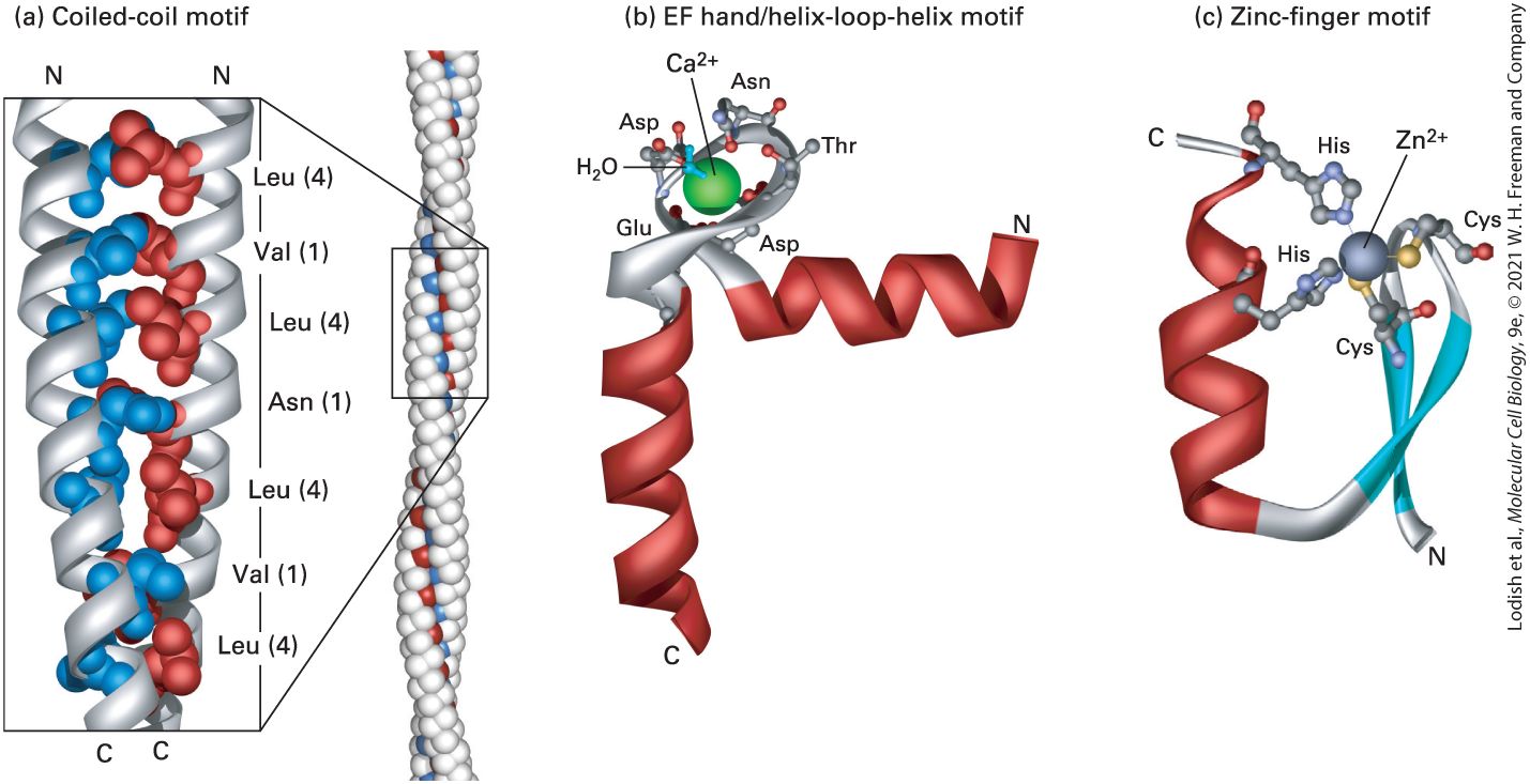
or loops. Such predictions can be used to predict the consequences of a mutation in a gene on the encoded protein’s secondary structures, and possibly on its function. Structural Motifs Are Regular Combinations of Secondary Structures A particular combination of two or more secondary structures that forms a distinct three-dimensional structure, which appears in multiple proteins, is called a structural motif. A structural motif — an alternative name is supersecondary structure — is often associated with a specific function, such as binding to a particular ion or small molecule, such as calcium or ATP. Some structural motifs are stable after being isolated from the rest of a protein and are thus called structural domains, as we shall see shortly. However, other structural motifs do not form thermodynamically stable structures in the absence of other portions of the protein and are thus not considered independent structural domains. One common structural motif is the α helix–based coiled coil. In this motif, α helices from two, three, or even four separate polypeptide chains coil about one another — resulting in a coil of coils; hence the name (Figure 3-7a). Many proteins, including fibrous proteins and DNAregulating proteins called transcription factors (see Chapter 8) assemble into dimers or trimers by using a coiled-coil motif. The individual helices bind tightly to one another because each helix has a strip of aliphatic

(hydrophobic, but not aromatic) side chains (leucine, valine, etc.) running along one side of the helix that interacts with a similar strip in the adjacent helix, thus sequestering the hydrophobic groups away from water and stabilizing the assembly of multiple independent helices. These hydrophobic strips are generated along only one side of the helix because the primary structure of each helix is composed of repeating seven–amino acid units, called heptads or heptad repeats, in which the side chains of the first and fourth residues are aliphatic and the other side chains are often hydrophilic (see Figure 3-7a). Because hydrophilic side chains extend from one side of the helix and hydrophobic side chains extend from the opposite side, the overall helical structure is amphipathic. Because leucine frequently appears in the fourth positions and the hydrophobic side chains merge together like the teeth of a zipper, these structural motifs are also called leucine zippers. A heptad repeat is an example of a sequence motif, a pattern of amino acids in a contiguous segment of a protein that can be found in many proteins, and sometimes in many copies within one protein. The sequence motif may be either an exact copy of the same sequence in every protein or a pattern of similar residues that do not have precisely the same sequence, such as the common spacing of aliphatic residues in a heptad repeat. Many different structural motifs contain α helices. A common calciumbinding motif called the EF hand contains two short α helices connected by a loop (Figure 3-7b). This structural motif, one of several helix-turnhelix and helix-loop-helix structural motifs, is found in more than a

hundred proteins and is used for sensing calcium levels. ion binds to oxygen atoms in conserved residues in the loop when the concentration of in the cell is high enough. Sometimes the binding induces a conformational change in the protein bearing the EF hand, altering the protein’s activity. Thus calcium concentrations can directly control the structures and functions of certain proteins. Somewhat different helixturn-helix and basic helix-loop-helix (bHLH) structural motifs are used for protein binding to DNA and, consequently, for the regulation of gene activity (see Chapter 8). Yet another structural motif commonly found in proteins that bind RNA or DNA is the zinc finger. This motif contains three secondary structures — an α helix and two β strands with an antiparallel orientation — that form a fingerlike bundle held together by a zinc ion (Figure 3-7c).

FIGURE 3-7 Motifs of protein secondary structure. (a) This parallel, two-stranded coiledcoil motif (left) is characterized by two α helices wound around each other. The backbone of the residues is represented as a ribbon, as illustrated in Figure 3-4, with atoms of only

some of the side chains represented as balls. Helix packing is stabilized by interactions between hydrophobic side chains (red and blue) present at regular intervals along each strand and found along the seam of the intertwined helices. Each α helix exhibits a characteristic heptad repeat sequence with a hydrophobic residue often, but not always, at positions 1 and 4, as indicated. The coiled-coil nature of this structural motif is more apparent in long coiled coils containing many such sequence motifs (right). (b) An EF hand, a type of helix-loop-helix motif, consists of two helices connected by a short loop in a specific conformation. The backbone of the residues is represented as a ribbon with only some of the side chains represented as balls (atoms) and sticks (bonds). This structural motif is common to many proteins, including many calcium-binding and DNA-binding regulatory proteins. In calcium-binding proteins such as calmodulin, oxygen atoms from five residues in the acidic glutamate- and aspartate-rich loop and one water molecule form ionic bonds with a large ion (green). (c) The zinc-finger motif is present in many DNA-binding proteins that help regulate transcription. A ion is held between a pair of β strands (blue) and a single α helix (red) by a pair of cysteine residues and a pair of histidine residues. The two invariant cysteine residues are usually at positions 3 and 6, and the two invariant histidine residues are at positions 20 and 24 in this 25-residue motif. [Part (a) Data from L. Gonzalez, Jr., D. N. Woolfson, and T. Alber, 1996, Nat. Struct. Biol. 3:1011–1018, PDB IDs 1zik and 2tma. Part (b) Data from R. Chattopadhyaya et al., 1992, J. Mol. Biol. 228:1177–1192, PDB ID 1cll. Part (c) Data from S. A. Wolfe, R. A. Grant, and C. O. Pabo, 2003, Biochemistry 42:13401–13409, PDB ID 1llm.] Description In illustration a, coiled-coil motif shows two alpha-helices tightly wound around each other. Each helix is made of several tightly bound white spheres with blue and red spheres present where both helices are in contact with each other. An enlarged view of a small section shows the close-up arrangement of the polypeptide chain labeled from top N-terminus to bottom C-terminus: Leu (4), Val (1), Leu (4), Asn (1), Leu (4), Val (1), and Leu (4). In illustration b, E F hand or helix-loop-helix motif shows a loop in between two helical structures. A large sphere of calcium (C A superscript 2 positive) is present in the loop with a water (H subscript 2 O) molecule attached to it. An arrangement of the

polypeptide chain labeled from N-terminus to C-terminus is as follows: Asp, Asp, Asn, Thr, and Glu. In illustration c, zinc-finger motif shows a helical structure attached to two beta-strands forming a U-shape. A large sphere of zinc (Z n superscript 2 positive) is attached at the top of the U-shaped structure and bonded to His on helical strand and two Cys on betastrands. Another His molecule is present toward the top C-terminus of the helical strand. The relationship between the primary structure of a polypeptide chain and the structural motif into which a portion of it folds is not always straightforward. The amino acid sequences responsible for any given structural motif in different proteins may be very similar to one another. In other words, a common sequence motif can result in a common structural motif. This is the case for the heptad repeats that form coiled coils. However, it is also possible for seemingly unrelated amino acid sequences to fold into a common structural motif, so it is not always possible to predict which amino acid sequences will fold into a given structural motif. Conversely, it is possible that a commonly occurring sequence motif will not fold into a well-defined structural motif. Sometimes short sequence motifs that have an unusual abundance of a particular amino acid, such as proline or aspartate or glutamate, are called domains; however, these and other short contiguous segments are more appropriately called sequence motifs than domains, as the latter term has a distinct meaning that we will define shortly. We will encounter numerous additional motifs in our discussions of proteins in this and other chapters. The presence of the same structural

Tertiary Structure Is the Overall Folding of a Polypeptide Chain

motif in different proteins with similar functions clearly indicates that these useful combinations of secondary structures have been conserved in evolution. Tertiary Structure Is the Overall Folding of a Polypeptide Chain Tertiary structure refers to the overall conformation of a polypeptide chain — that is, the three-dimensional arrangement of all its amino acid residues. In contrast to secondary structures, which are stabilized only by hydrogen bonds, tertiary structure is stabilized primarily by hydrophobic interactions between nonpolar side chains, together with van der Waals interactions and hydrogen bonds involving both polar side chains and backbone amino and carboxyl groups. These stabilizing forces hold together elements of secondary structure — α helices, β strands, turns, and loops — and structural motifs. Because the interactions stabilizing tertiary structures are often weaker than those stabilizing secondary structure, the tertiary structure of a protein is not necessarily rigidly fixed, but can undergo continual minute fluctuations. Some segments within the tertiary structure of a protein can be so mobile that they are considered to be disordered — that is, lacking a single, well-defined, stable, threedimensional structure. This variation in structure has important consequences for the function and regulation of proteins. The chemical properties of amino acid side chains help define tertiary structure. In some proteins — for example, those that are secreted from

cells or are cell-surface proteins that face the extracellular environment — disulfide bonds form between the side chains of cysteine residues. Disulfide bonds can covalently link regions of the proteins, thus restricting the proteins’ flexibility and increasing the stability of their tertiary structures. Amino acids with charged hydrophilic polar side chains tend to be on the outer surfaces of water-soluble proteins; by interacting with water, they increase the protein’s solubility in water. Moreover, these polar side chains can form noncovalent interactions with other water-soluble molecules, including other proteins. In contrast, amino acids with hydrophobic nonpolar side chains are usually sequestered away from the water-facing surfaces of a protein, in many cases forming a waterinsoluble central core. This observation led to what’s known as the oil drop model of protein conformation because the core of a protein is relatively hydrophobic, or oily (Figure 3-8). Hydrophilic polar side chains that are uncharged are found both on the surface and in the inner core of water-soluble proteins.

FIGURE 3-8 The oil drop model of protein folding. The hydrophobic and hydrophilic residues of a polypeptide chain can be distributed throughout its linear sequence as illustrated in the unfolded protein (top). The color scale denotes the most hydrophilic residues (blue) to the most hydrophobic (yellow). When the protein folds (bottom left), hydrophilic (charged and uncharged polar) side chains will often be exposed on the protein’s surface, where they can form stabilizing interactions with surrounding water and ions. In contrast, the hydrophobic residues tend to cluster together in the inner core, somewhat like drops of oil in an aqueous liquid, driven away from the aqueous surroundings by the hydrophobic effect (see Chapter 2). These core residues are more easily seen when several surface residues are removed (bottom right). [Data from M. C. Vaney et al., 1996, Acta Crystallogr., Sect. D. 52:505, PDB ID 193l.]

Different Ways of Depicting the Conformation of Proteins Convey Different Types of Information

Description A color-coded scale at the top is labeled most hydrophilic toward the left blue end and most hydrophobic toward the right yellow end. The color shade changes from left to right with green in the center. An unfolded linear-shaped protein structure shows random arrangement of blue, green, and yellow color residues from N to C terminus. After the folding process, this results in the formation of a folded oval-shaped protein structure with blue and green color residues lying on the surface. After removing several surface residues to reveal protein’s core, it shows the core or the center made of yellow color residues. The folding process is reversible wherein unfolding process may convert folded protein to unfolded protein. As you might expect, our ability to predict the tertiary structure for most proteins from primary sequence is not as advanced as our ability to predict secondary structure from sequence. One method to assess the quality of a tertiary structure prediction is to use the total score of the global distance test (a scale from 0 to 100), which compares the prediction with an experimentally determined structure. A score of is a clearly incorrect prediction, scores of 80–90 are close to identifying the positions of individual atoms, and 100 is perfect. Current methods result in predictions around 57, which provide a good representation of the overall chain folding, but often have serious errors when compared to experimental results. At this time, predictions are better for shorter (length residues) polypeptides. Different Ways of Depicting the Conformation of Proteins Convey

Different Types of Information The simplest way to represent three-dimensional protein structure is to trace the course of the backbone atoms, sometimes only the atoms, with a solid line — or narrow tube — called a backbone trace (Figure 3-9a); the most complex representation, called a ball-and-stick model, shows every atom (Figure 3-9b). The backbone trace shows the overall folding of the polypeptide chain without consideration of the amino acid side chains; the ball-and-stick model (with balls representing atoms and sticks representing bonds) details the interactions between side-chain atoms, including those that stabilize the protein’s conformation and interact with other molecules, as well as the atoms of the backbone. Even though both views are useful, the elements of secondary structure are not always easily discerned in them. Another type of representation, called a ribbon diagram, uses common shorthand symbols for depicting secondary structure — for example, coiled ribbons or solid cylinders for α helices, flat ribbons or arrows for β strands, and flexible thin strands for β turns, coils, and loops (Figure 3-9c). In a variation of the basic ribbon diagram, ball-and-stick or space-filling models of side chains are attached to the backbone ribbon, as we have seen in Figure 3-7. In this way, side chains of interest can be visualized clearly in the context of the secondary structure that is represented by the ribbons.

FIGURE 3-9 Five ways to visualize the protein Ras with its bound GDP. (a) The backbone trace demonstrates how the polypeptide is tightly packed into a small volume. (b) A ball-and-stick representation reveals the locations of all atoms. (c) Turns and loops connect pairs of helices and strands. (d) A water-accessible surface reveals the numerous lumps, bumps, and crevices on the protein surface. Regions of positive charge are shaded blue, and regions of negative charge are shaded red. (e) Hybrid model combines ribbon and transparent surface models. [Data from E. F. Pai et al., 1990, EMBO J. 9:2351–2359, PDB ID 5p21.] Description In illustration a, C subscript alpha backbone trace shows several alpha-helices joined to beta-sheets with a ball-and-stick G D P molecule. In illustration b, ball-and-stick model shows a cluster of alpha-helices joined to beta-sheets with a G D P molecule at the top left surface. In illustration c, ribbon diagram shows ribbon-like alpha-helices joined to thread-like beta-sheets forming several turns and loops. A ball-and-stick G D P molecule is bound at the top left. In illustration d, water accessible surface shows a color-coded oval-shaped structure with an irregular surface. Random patches of red,

Domains Are Modules of Tertiary Structure

blue, and white colors in equal quantity forms the structure with a ball-and-stick G D P molecule present at the top left. In illustration e, hybrid model shows a white-color oval-shaped structure with an irregular surface. The structure shows a ribbon diagram inside it. However, none of these three ways of representing protein structure conveys much information about the atoms that are on the protein’s surface and in contact with the protein’s environment. The surface is of interest because it is where other molecules usually bind to a protein. Thus a useful alternative way to represent proteins is to show only the surface and use colors to highlight regions having a common chemical character, such as hydrophobicity or hydrophilicity, and charge characteristics, such as positive (basic) or negative (acidic) side chains (Figure 3-9d). Such models reveal the topography of the protein surface and the distribution of charge, both important features of binding sites, as well as clefts in the surface where other molecules may bind. This view represents a protein as it is “seen” by other molecules. Hybrid models (Figure 3-9e) combine features of multiple types of protein representation. Domains Are Modules of Tertiary Structure Distinct regions of protein structure are often referred to as domains. There are three main classes of protein domains: functional, structural, and topological. A functional domain is a region of a protein that exhibits a particular activity characteristic of that protein, usually even when

isolated from the rest of the protein. For instance, a particular region of a protein may be responsible for a catalytic activity (e.g., a kinase domain that covalently adds a phosphate group to another molecule) or its binding ability (e.g., a DNA-binding domain or a membrane-binding domain). Functional domains are often identified experimentally by whittling down a protein to its smallest active fragment with the aid of proteases, enzymes that cleave one or more peptide bonds in a target polypeptide. Alternatively, the DNA encoding a protein can be modified so that when the modified DNA is used to generate a protein, only a particular region, or domain, of the full-length protein is made. Thus it is possible to determine if specific parts of a protein are responsible for particular activities exhibited by the protein. Indeed, functional domains are often also associated with corresponding structural domains. A structural domain is a region about 40 or more amino acids in length, arranged in a single, stable, and distinct structure often comprising one or more secondary structures or structural motifs. Many structural domains can fold into their characteristic structures independently of the rest of the protein in which they are embedded. As a consequence, distinct structural domains can be linked together — sometimes by stretches of polypeptide chain called spacers — to form a large multidomain protein (somewhat like beads on a string). Each of the polypeptide chains in the trimeric flu virus hemagglutinin, for example, contains a globular domain and a fibrous domain (Figure 3-10a).

FIGURE 3-10 Tertiary and quaternary levels of structure. The protein pictured here, hemagglutinin (HA), is found on the surface of the influenza virus. This long molecule has three identical subunits, each composed of two polypeptide chains, and . (a) The tertiary structure of each HA subunit comprises the folding of its helices and strands into a compact structure that is 13.5 nm long and divided into two domains. The membranedistal domain (silver) is folded into a globular conformation. The membrane-proximal domain (gold) has a fibrous, stemlike conformation owing to the alignment of two long α helices (cylinders) of with β strands in . Short turns and longer loops, many of them at the surface of the molecule, connect the helices and strands in each chain. (b) The quaternary structure of HA is stabilized by lateral interactions between the long helices

(cylinders) in the fibrous domains of the three subunits (gold, blue, and green), forming a triple-stranded coiled-coil stalk. Each of the distal globular domains in HA binds sialic acid (red) on the surface of target cells. Like many membrane proteins, HA contains several covalently linked carbohydrate chains (not shown). [Data from S. J. Gamblin et al., 2004, Science 303:1838–1842, PDB ID 1ruz.] Description In illustration a, the tertiary structure shows two H A subunits, a proximal H A subscript 1 and distal H A subscript 2. The H A subscript 1 labeled fibrous domain has elongated structure with long alpha-helix strands while the H A subscript 2 labeled globular domain has a globular structure with shorter alpha-helix strands. The proximal end lies above the external surface of the viral membrane with C-terminus entering the internal surface. In illustration b, the quaternary structure shows a cluster of three H A subunits attached to each other. Each subunit is formed of an elongated proximal domain and globular distal domain. One sialic acid molecule is bound to each distal subunit. Structural domains frequently are also functional domains in that they can have an activity independent of the rest of the protein. Structural domains can be incorporated as modules into different proteins. The modular approach to protein architecture is particularly easy to recognize in large proteins, which tend to be mosaics of different domains that confer distinct activities and thus can perform different functions simultaneously. As many as 80 percent of the proteins in eukaryotes have multiple structural domains. The organization (order) of domains within a multidomain protein is called the domain architecture. A useful simile is that a protein is like a sentence. The amino acid residues are like letters, spaces, and punctuation marks, and the structural domains are like words,

each having its distinct activity, and, when joined together into a sentence, they generate a protein with a distinctive function. Thousands of structural domains have been identified in proteins. Some of these are not very common, whereas others are found in many different proteins. Indeed, by some estimates, only nine major types of structural domains account for as much as a third of all the structural domains in all proteins. Structural domains can be recognized in proteins whose structures have been determined by x-ray crystallography or nuclear magnetic resonance (NMR) analysis or in images captured by electron microscopy (see Section 3.5). For example, the epidermal growth factor (EGF) domain is a structural domain that is present in several proteins (Figure 3-11). EGF is a small, soluble peptide hormone that binds to cells in the embryo and in skin and connective tissue in adults, causing them to divide. It is generated by proteolytic cleavage (breaking of a peptide bond) between repeated EGF domains in the EGF precursor protein, which is anchored in the plasma membrane by a membrane-spanning domain. EGF domains with sequences similar to, but not identical to, that of the EGF peptide hormone are present in other proteins and can be liberated by proteolysis. These proteins include tissue plasminogen activator (TPA), a protease that is used to dissolve blood clots in heart attack victims; Neu protein, which takes part in embryonic differentiation; and Notch protein, a receptor protein in the plasma membrane that functions in signaling and is important for development (see Chapter 16). Besides the EGF domain, these three proteins have other domains in common with other proteins. For example, TPA possesses a trypsin domain, a functional domain found in some proteases.

FIGURE 3-11 Modular nature of protein domains. Epidermal growth factor (EGF) is generated by proteolytic cleavage of a precursor protein containing multiple EGF domains (green) and a membrane-spanning domain (blue). An EGF domain is also present in the Neu protein and in tissue plasminogen activator (TPA). These proteins also contain other widely distributed domains, indicated by shape and color. See I. D. Campbell and P. Bork, 1993, Curr. Opin. Struc. Biol. 3:385. Description The first protein E G F precursor is made of a chain of nine green spheres attached to a blue rectangle. The Neu protein is made of a grey Y-shaped structure attached to a green sphere which is further attached to a blue rectangle. The E G F protein is made of a single green sphere. The T P A protein is made of a small pink oval attached to a green sphere attached to an orange square attached to another orange square which is finally attached to a large yellow oval. Regions of proteins that are defined by their distinctive spatial relationships to the rest of the protein are topological domains. For example, some proteins associated with cell-surface membranes have a part extending inward into the cytoplasm (cytoplasmic domain), a part embedded within the phospholipid bilayer (membrane-spanning domain),

Comparing Protein Sequences and Structures Provides Insight into Protein Function and Evolution

and a part extending outward into the extracellular space (extracellular domain). Each of these topological domains can comprise one or more structural and functional domains. It is also common for the region of a protein at the N-terminus or C-terminus to be called the N-terminal or C-terminal domain, respectively. In Chapter 7, we will consider the mechanism by which the gene segments that correspond to domains became shuffled in the course of evolution, resulting in their appearance in many proteins. Once a functional, structural, or topological domain has been identified and characterized in one protein, it is possible to use that information to search for similar domains in other proteins and to suggest potentially similar functions for those domains in those proteins. Comparing Protein Sequences and Structures Provides Insight into Protein Function and Evolution Analyses of many diverse proteins have conclusively established a relation between the amino acid sequence, three-dimensional structure, and function of proteins. A good rule of thumb is that the greater the similarity of the sequences of two polypeptide chains, the more likely they are to have similar three-dimensional structures and similar functions. Although this comparative approach is very powerful, caution must always be exercised when attributing to one protein, or a part of a protein, a function or structure similar to that of another protein based only on amino acid

sequence similarities. There are examples in which proteins with similar overall structures display different functions, as well as cases in which proteins unrelated in amino acid sequence or function nevertheless have very similar folded tertiary structures. In many cases, however, such sequence comparisons provide important insights into protein structure and function. Investigators have increased the use of protein sequence comparisons to study protein structure and function as the genomes and transcriptomes of more and more organisms are sequenced, because a vast array of protein sequences has been deduced from the nucleic acid sequences. Indeed, the molecular revolution in biology during the last decades of the twentieth century created a new scheme of biological classification based on similarities and differences in the amino acid sequences of proteins. Proteins that have a common ancestor are referred to as homologs. The main evidence for homology among proteins, and hence for their common ancestry, is similarity in their sequences, which is often reflected in similar structures. We can describe homologous proteins as belonging to a family and can trace their lineage — how closely or distantly they are related to one another in an evolutionary sense — from comparisons of their sequences. Generally more closely related proteins exhibit greater sequence similarity than more distantly related proteins because, over evolutionary time, alterations in the DNA sequences accumulate in the genes encoding these proteins. The folded threedimensional structures of homologous proteins may be similar even if some parts of their primary structure show little evidence of sequence homology.

Based on their sequences, structural similarities, evolutionary histories and functions, related proteins have been classified as belonging to hierarchical sets of proteins called superfamilies, groups, subgroups, families, and subfamilies. The sequences of members of each subfamily are more similar to each other than they are to those of members of other subfamilies within the same family. Initially, proteins with relatively high sequence similarities ( percent exact amino acid matches, or identities) and related functions or structures were defined as an evolutionarily related family, while a superfamily encompassed two or more families in which the interfamily sequences matched less well ( percent identities) than within one family. It is generally thought that proteins with about 30 percent sequence identity are likely to have similar three-dimensional structures; however, such high sequence identity is not required for proteins to share similar structures. The kinship among homologous proteins is most easily visualized by a tree diagram (in essence, a family tree) based on sequence analyses. For example, the amino acid sequences of globins — the proteins hemoglobin and myoglobin and their relatives from bacteria, plants, and animals — suggest that they evolved from an ancestral monomeric oxygen-binding protein (Figure 3-12a). With the passage of time, the gene for this ancestral protein slowly changed due to random changes in the DNA sequence, initially diverging into lineages leading to animal and plant globins. Subsequent changes gave rise to myoglobin and, after a gene duplication, to the α and β subunits of the tetrameric hemoglobin molecule of the vertebrate circulatory system.

FIGURE 3-12 Evolution of protein families. (a) A primitive monomeric oxygen-binding globin is thought to be the ancestor of modern-day blood hemoglobins, muscle myoglobins, and plant leghemoglobins. Sequence comparisons have revealed that the evolution of the globin proteins parallels the evolution of animals and plants. Major changes occurred with the divergence of plant globins from animal globins and of myoglobin from hemoglobin. Later, gene duplication gave rise to the α and β subunits of hemoglobin. See R. C. Hardison, 1996, Proc. Nat’l. Acad. Sci. USA 93:5675. (b) The family tree of 478 human protein kinases is divided into seven major groups of protein kinase families (comprising 405 kinases), designated: CMGC, CAMK, AGC, CK1, STE, TKL, and TK. Each of these contains families and subfamilies. We will describe the critical roles of kinases from many of these groups in subsequent chapters. For example, the members of the TK (tyrosine kinase) group are distinctive because they phosphorylate the side chains of tyrosine residues. One TK member is the receptor for the hormone insulin (Chapter 16). [Part (b) Republished with permission of American Association for the Advancement of Science, from G. Manning et al., 2002, “The Protein Kinase Complement of the Human Genome,” Science 298:1912–1934; permission conveyed through Copyright Clearance Center, Inc.] Description

In illustration a, the evolutionary tree starting with an ancestral oxygen-binding protein shows the main branch branching out into three sub branches. The first sub branch leads to bacterial, second to fungal, and third bifurcates into algal and protozoan. The main branch splits into two major branches. The first major branch, sub branches into nematode, annelid, and insect; and finally splits into two: one leads to myoglobin and the other bifurcates into alpha hemoglobin and beta hemoglobin in the vertebrate. The second major branch splits into dicot hemoglobin and the other bifurcates into leghemoglobin and monocot hemoglobin. In illustration b, the family tree of 478 human protein kinases is divided into 7 major groups. A multi-branched tree with a center leads to 7 sets of color-coded branches having several tiny branches. From the top in clockwise direction, these groups are labeled: T K L, S T E, C K 1, A G C, C A M K, C M G C, and T K. A series of duplications and divergences can lead to the generation of a large, highly branched family of genes and corresponding proteins within a single organism. Figure 3-12b shows such a family tree for the 478 human protein kinase enzymes that evolved from one ancient precursor. All of these kinases catalyze the covalent addition of a phosphate group from ATP to the hydroxyl group of the side chains of serine, threonine, or tyrosine ( percent phosphorylate tyrosines) (see Figure 2-15). A small number phosphorylate both serine (or threonine) and tyrosine are called dual-specificity kinases. Forty additional human kinases evolved from other precursors, and thus there is a total of 518 kinases in what is called the human kinome. In such a large family tree, the sum of the lengths of the lines between one member and another is generally proportional to the evolutionary distance between the two proteins — the shorter the distance on the tree between any two members of the family, the more similar they are in sequence and typically in structure and function. Often analysis of the branching patterns of proteins in such family trees is used to subdivide

There Are Four Broad Structural Categories of Proteins

the members into groups, families, and subfamilies (Figure 3-12b) rather than relying on a precise formula using an arbitrary percent identity of sequence to define subfamilies, families, and so on. There Are Four Broad Structural Categories of Proteins Proteins usually fall into one of four broad structural categories based on their tertiary structure: globular proteins, fibrous proteins, integral membrane proteins, and intrinsically disordered proteins. These four broad categories of proteins are not mutually exclusive — some proteins are made up of combinations of segments that fall into two or more of these categories. Globular proteins are generally water-soluble, compactly folded structures, often spheroidal, that comprise a mixture of secondary structures (e.g., see Figure 3-9). Fibrous proteins are large, elongated, often stiff molecules. Some fibrous proteins are composed of a long polypeptide chain comprising many tandem copies of a short amino acid sequence motif that forms a single repeating secondary structure. These fibrous proteins are often made up of helical polypeptide chains, including α helices, triple helices (see the structure of collagen, the most abundant protein in mammals, in Figure 20-26) and helical coil coils with two or more strands (see Figure 3-7). Other fibrous proteins are composed of repeating globular protein subunits, such as the helical array of G-actin protein monomers that forms F-actin microfilaments (see Chapter 17). Fibrous proteins, which can aggregate into large multiprotein fibers that do not readily dissolve in water, usually play a structural role or

participate in cellular movements. Integral membrane proteins are embedded within the phospholipid bilayer of the membranes that enclose cells and organelles. Their membrane-spanning domains often comprise one or more -residue long α helices and occasionally β barrels; they are discussed in detail in Chapter 10. Regardless of a protein’s category of tertiary structure, one or more segments of the protein may be disordered meaning that they do not form thermodynamically stable structures. Disordered protein segments are exceptionally flexible in conformation, and their flexibility appears to be key to their functional activities. Regions of disorder can provide flexible links, or tethers, between well-ordered regions of a protein; serve as binding sites for other proteins (Figure 3-13a); serve as sites of some types of post-translational protein modification [e.g., covalent addition of phosphate groups (phosphorylation) or sugars (glycosylation)]; serve as targets of protease digestion that regulates protein activity; inhibit the activity of the protein in which they are embedded (autoinhibition sites); or serve as signals for intracellular sorting of proteins (see Chapter 13). The activities of many proteins containing disordered segments are described in subsequent chapters. For example, phosphorylation of the disordered C-terminal domain (CTD) of RNA polymerase II (see Figure 812), which is composed of multiple repeats of a seven–amino acid sequence containing proline, threonine, and serine, regulates key steps in the synthesis of mRNA (see Chapters 8 and 9). The N-termini of histone proteins that control DNA organization in chromatin (see Chapter 7) are sites of important post-translational modifications, and the disordered,

proline-rich FH1 region in the protein formin controls the assembly of actin filaments (see Chapter 17). Many proteins we consider in this book adopt only one or a few very closely related conformations when they are in their normal functional state, called the native state. However, in some proteins, the entire polypeptide chain is disordered. These proteins do not have well-ordered structures in their native, functional states; instead, their polypeptide chains are very flexible with no fixed conformation. These proteins are called intrinsically disordered proteins (IDP). Intrinsically disordered proteins typically serve as signaling molecules, regulators of the activities of other molecules, or as scaffolds for multiple proteins, small molecules, and ions (e.g., binding ions via multiple charged residues). Disordered segments may also be present in otherwise well-structured proteins; these disordered segments are called intrinsically disordered regions (IDR). Intrinsically disordered proteins and disordered segments can be identified experimentally using various biochemical techniques, such as tests of sensitivity to protease digestion (disordered regions usually exhibit greater protease sensitivity), and a wide variety of biophysical techniques, including spectroscopy. The disorder of these protein segments or of an entire protein apparently arises as a consequence of their having a sequence that, relative to well-ordered proteins, is richer in polar amino acids, proline, and net charge, and poorer in hydrophobic residues (Figure 3-13b). Algorithms primarily based on calculations of amino acid composition — particularly net charge and hydrophobicity — are used to predict which proteins or segments of proteins are disordered. By some

estimates, about 30 percent or more of eukaryotic proteins have at least one segment of 50 or more consecutive residues that is disordered. In some cases, an intrinsically disordered protein (or region) can transition into a highly ordered structure (see Figure 3-13a). EXPERIMENTAL FIGURE 3-13 Intrinsically disordered proteins: mechanisms of binding to well-ordered proteins and identification based on hydrophobicity and net charge. (a) The binding of an intrinsically disordered protein (PUMA, blue) to a wellordered protein (MCL1, gray) results in the formation of a well-defined structure in the previously disordered protein. Two mechanisms have been proposed for generating a bound complex in which both proteins are structured: conformational selection (top pathway) and induced fit (bottom pathway). In conformational selection, the disordered protein (PUMA) occasionally and transiently adopts in solution the structure it would have in the bound state. The well-ordered binding partner (MLC1) can then bind to (select) PUMA in that transient, ordered conformation, forming a relatively stable bound complex. In induced fit, the disordered protein begins to bind to the well-ordered partner while still disordered and then, while bound, is induced to form the ordered conformation present in the relatively stable, heterodimeric complex. Experiments suggest that the induced fit mechanism best describes the binding of PUMA and MCL1. (b) The sequences of 275 well-ordered, monomeric globular proteins (gray squares) and 91 intrinsically disordered proteins (black and yellow circles) were used to calculate the mean hydrophobicity per residue in each protein using a scale of 0 (least hydrophobic) to 1 (most hydrophobic, x axis), and the mean

Multiple Polypeptides Assemble into Quaternary Structures, Supramolecular Complexes, and Biomolecular Condensates

net charge per residue at pH 7.0 (y axis). With only three exceptions (black circles), the proteins define two distinct distributions: low hydrophobicity, high net charge (intrinsically disordered, yellow circles) and high hydrophobicity, low net charge (well-ordered, gray squares). The three disordered proteins (black circles) that overlap with the well-ordered population each contain substantial segments predicted to be disordered (low hydrophobicity, high net charge) that apparently overwhelm the rest of the proteins’ sequences that might otherwise result in a well-ordered conformation. [Part (a) From J. M. Rogers, A. Steward, and J. Clarke, 2013, “Folding and Binding of an Intrinsically Disordered Protein: Fast, but Not ‘Diffusion-Limited,’ ” J. Am. Chem. Soc. 135(4):1415–1422; https://doi.org/10.1021/ja309527h. Part (b) Data from V. N. Uversky, J. R. Gillespie, and A. L. Fink, 2000, Proteins 41:415–427.] Description The illustration labeled (a) shows a helical, linear transiently ordered P U M A attaching to a globular, helical well-structured M C L 1 by conformation selection; and three thread-like intrinsically disordered P U M As attaching to an M C L 1 by induced fit. Both attachments lead to the formation of an ordered P U M A bound to M C L 1. In the scatterplot labeled (b), the horizontal axis represents mean hydrophobicity and ranges from 0.1 to 0.6 in increments of 0.1. The vertical axis represents mean net charge and ranges from 0.0 to 0.6, in increments of 0.2. A dashed line starts from (0.4, 0.0) and ends at (0.6, 0.55). Majority of the well structured units are present on the right side of the dashed line, between 0.4 and 0.55 on the horizontal axis and between 0.0 and 0.15 on the vertical axis. Majority of the intrinsically disordered units are present on the left side of the dashed line, between 0.3 and 0.4 on the horizontal axis and between 0.0 and 0.2 on the vertical axis. The three exception units lie on the right side of the dashed line, between 0.4 and 0.45 on the horizontal axis and between 0.0 and 0.1 on the vertical axis. All data are approximate. Multiple Polypeptides Assemble into Quaternary Structures,

Supramolecular Complexes, and Biomolecular Condensates Multimeric proteins consist of two or more polypeptide chains that in this context are referred to as subunits. A fourth level of structural organization, quaternary structure, describes the number (stoichiometry), relative positions, and often the tertiary structures of the subunits in multimeric proteins. Multimeric proteins are composed of various numbers of identical (homomeric) or different (heteromeric) subunits, typically held together by noncovalent bonds. Flu virus hemagglutinin, for example, is a trimer of three identical subunits (a homotrimer) (see Figure 3-10). In many cases, the individual monomer subunits of a multimeric protein cannot function normally unless they are assembled into the multimeric protein. In other cases, assembly into a multimeric protein permits proteins that act sequentially in a pathway to increase their efficiency of operation owing to their juxtaposition in space, a phenomenon referred to as metabolic coupling. Classic examples of metabolic coupling are the fatty acid synthases of fungi, which are enzymes that synthesize fatty acids, and the polyketide synthases, which are large multiprotein complexes in bacteria that synthesize a diverse set of molecules called polyketides often used as drugs, including the antibiotic erythromycin. Supramolecular Complexes

The highest level in the hierarchy of protein structure is the association of proteins into supramolecular complexes. Typically, such structures are very large, containing tens to hundreds of polypeptide chains and sometimes other biopolymers such as nucleic acids. In some cases, supermolecular structures exceed 1 megadalton (MDa) in mass, approaching 30–300 nm in size. The capsid that encases the nucleic acids of a viral genome is an example of a supramolecular complex with a structural function. The bundles of cytoskeletal filaments that support and give shape to the plasma membrane are another example. Other supramolecular complexes act as molecular machines. These complexes carry out complex cellular processes by integrating multiple proteins, each with distinct functions, into one large assembly. For example, a transcriptional machine is responsible for synthesizing messenger RNA (mRNA) using a DNA template. The operational details of this transcriptional machine are discussed in Chapters 5 and 8. It consists of RNA polymerase, itself a multimeric protein, and at least 50 additional components, including general transcription factors, promoterbinding proteins, helicase, and other protein complexes (Figure 3-14). Ribosomes, also discussed in Chapter 5, are complex machines that synthesize proteins and are formed of multiple proteins and nucleic acids. One of the most complex multiprotein assemblies is the nuclear pore, a structure that allows macromolecules to pass between the nucleus and the cytoplasm (see Chapter 13). It is composed of multiple copies of about 30 distinct proteins and forms an assembly with an estimated mass of 50 MDa. The fatty acid synthases and polyketide synthases referred to above are also molecular machines, as is the mitochondrial supercomplex

that integrates multiple steps in the electron-transport chain that provides energy for synthesizing ATP. This supercomplex (Figure 12-23) comprises three supramolecular complexes and more than 64 polypeptide chains (see Chapter 12).

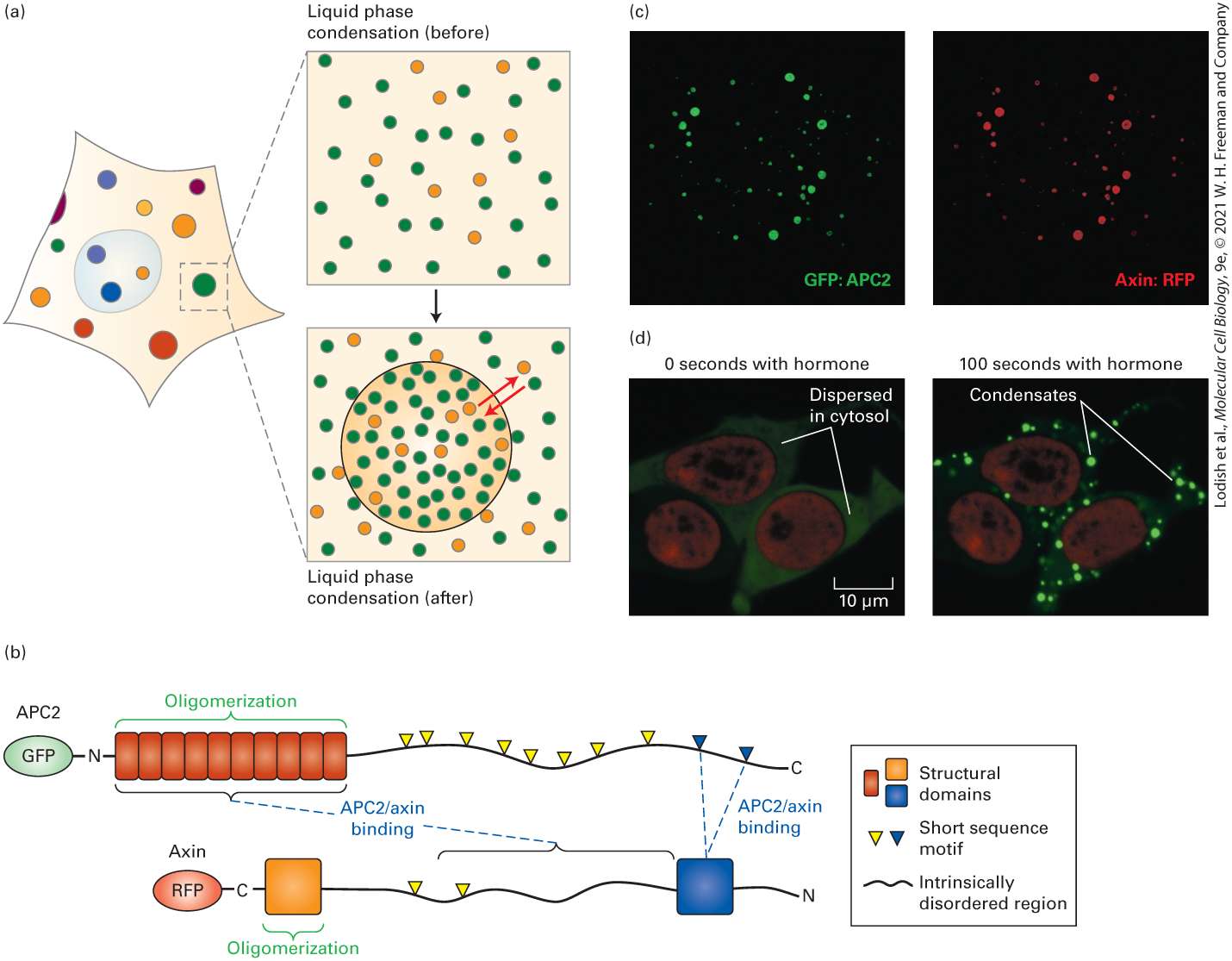
FIGURE 3-14 A molecular machine: the transcription initiation complex. The core RNA polymerase, general transcription factors, a mediator complex containing about 20 subunits, and other protein complexes not depicted here assemble at a promoter in DNA prior to the synthesis of the corresponding RNA. The polymerase carries out transcription of DNA; the associated proteins are required for initial binding of the polymerase to a specific promoter. Note that the DNA is bent in the transcription preinitiation complex. The multiple components function together as a molecular machine. Description The first step shows an R N A polymerase plus several subunits of general transcription factors plus a mediator complex plus a promoter site on a linear double-helical D N A. This leads to the formation of the transcription initiation complex wherein the doublehelical D N A forms a V-shape with a bend at the promoter site. The R N A polymerase is attached to the promoter site and is surrounded by the general transcription factor subunits which are further surrounded by the mediator complex. Biomolecular Condensates A rather different approach to organizing together large collections of macromolecules is the generation of biomolecular condensates that are likely to play important roles in multiple aspects of cell biology. Biomolecular condensates are membraneless compartments in cells, often compared to liquid droplets, that are chemically and physically distinct from their surroundings. In biomolecular condensates, multiple copies of one or more macromolecules separate from the bulk surrounding fluid in a process called liquid-liquid phase separation. Through such phase separation, macromolecules, often proteins or proteins combined with RNAs, assemble or condense into a region of higher concentration than in

the bulk surrounding fluid of the cytosol or nucleoplasm (Figure 3-15). Unlike the supramolecular complexes described above, biomolecular condensates can vary in size (100s to 1000s of nanometers), and their components generally do not have a fixed stoichiometry or quaternary structural arrangement. EXPERIMENTAL FIGURE 3-15 Multivalent proteins with intrinsically disordered regions and other characteristics can assemble into biomolecular condensates. (a) Cells contain a variety of membraneless condensates, resembling liquid droplets, in the cytoplasm and nucleus (colored circles, left). Macromolecules (small circles in expanded rectangle before condensation, upper right) separate from the bulk surrounding fluid and concentrate in a biomolecular condensate due to liquid-liquid phase separation (large green circle after condensation, lower right). These macromolecules can diffuse into and out of the

condensate (red arrows). (b) Models of the fruit fly (Drosophila melanogaster) proteins APC2 and Axin, two large proteins that participate in the Wnt signaling pathway (see

Chapter 16). Many other species, including mammals, express APC2 and Axin homologues. These multivalent proteins contain domains (rectangles and squares), intrinsically disordered regions (black lines), and short sequence motifs (triangles) that perform key functions. The motifs designated by yellow triangles are involved with binding additional Wnt-associated signaling molecules (Chapter 16). When APC2 and Axin are synthesized in cultured cells with covalently attached fluorescent proteins (ovals), they can be visualized using confocal fluorescence microscopy (Chapter 4). Each protein can oligomerize into larger complexes via the domains indicated by green brackets. (c) When expressed together, APC2 and Axin bind to each other [sites of binding indicated by blue dotted lines in panel (b)] forming biomolecular condensates that contain both proteins (both colors found in all condensates of various sizes, green GFP:APC2 on the left, red Axin:RFP on the right). (d) Two multivalent, artificial proteins, one of which is fluorescent (green) and can be easily detected by microscopy, were expressed together in human cells. These two proteins, which reside in the cytoplasm, cannot bind to one another unless the fluorescent protein is phosphorylated by the enzyme Protein Kinase A (PKA, see Section 3.4 and

Chapter 15). In the absence of the hormone isoprenaline (left panel, 0 seconds with hormone), PKA is inactive, the two proteins do not bind to one another, and the green fluorescent protein is dispersed throughout the cytosol (left panel). In this condition, the proteins do not enter the nucleus (red ovals in the centers of the cells, the DNA was stained red by a fluorescently labeled DNA-binding protein called histone 2B, see Chapter 7). Addition of isoprenaline for 100 seconds (right panel) activates PKA, resulting in phosphorylation of the fluorescent protein, binding of the two proteins and formation in the cytosol of biomolecular condensates in which the proteins are concentrated (green dots that are brighter than the dispersed green in the left panel). [Panel (a) Data from Y. Shin and C. P. Brangwynne, 2017, Science 357(6357):eaaf4382. Panel (b) Data from Figure 1, M. I. Pronobis et al., 2017, Mol. Biol. Cell 28:41–53; and

Figure 3, K. N. Schaefer and M. Peifer, 2019, Dev. Cell 48(4):429–444. Panel (c) Photos courtesy of Xiaokun Shu, from Q. Zhang et al., 2018, Mol. Cell. (left); D. Yu et al., 2015, Nat. Methods (right). Panel (d) Republished with permission from Elsevier, Inc., from K. N. Shaefer and M. Peifer, 2019, “Wnt/Beta-Catenin Signaling Regulation and a Role for Biomolecular Condensates,” Dev. Cell. 48(4):429–444; permission conveyed through Copyright Clearance Center, Inc.]

Description The illustration labeled (a) shows a cell sparsely filled with circles of different colors and sizes. A small square region enclosing a large green colored circle is enlarged to show a before and after diagram of liquid phase condensation. In liquid phase condensation (before), several small green circles fill the square along with a few small yellow circles. In liquid phase condensation (after), the square encloses a large circle in the center. The large circle is densely packed with several small green colored circles and few small yellow colored circles. While outside the circle, the square is sparsely filled with green and yellow colored small circles. An arrow points to a yellow colored small circle from inside to outside of the large circle and another arrow points to a green colored small circle from outside to inside. The illustration labeled (b) shows different regions of A P C 2 and Axin proteins. In A P C 2: an oval G F P is bound to the N terminal of 10 tightly attached vertical rectangular subunits of structural domain, labeled oligomerization. The opposite side of this domain shows a long tail-like intrinsically disordered region with eight yellow inverted triangles, labeled short sequence motif, attached at the top at some distance followed by two blue inverted triangles. In Axin: an oval R F P is bound to the C terminal of a blue square labeled oligomerization. The opposite side of the square shows a long tail-like intrinsically disordered region with two yellow inverted triangles, labeled short sequence motif, at the top. The tail ends to meet another blue square. This square further has a short tail at the opposite side labeled N terminal. The oligomerization region of A P C 2 and the latter three-fourth intrinsically disordered region of Axin are collectively labeled “A P C 2 slash axin binding.” The two blue triangles of A P C 2 and the top side of the second blue square of Axin is collectively labeled “A P C 2 slash axin binding.” The illustration labeled (c) shows two micrographs of proteins. On the left, the G F P: A P C 2 micrograph shows several different sized dots of light green against a dark green background. On the right, the Axin: R F P micrograph shows similar dots in light red against a dark red background. The illustration labeled (d) shows two micrographs of a hormone in cell at different time periods. The micrograph on the left, labeled “0 seconds with hormone” shows hormone dispersed in the cytosol. The micrograph on the right, labeled “100 seconds

with hormone” shows brightly lit dots of hormone, labeled condensates, in the cytoplasm. A biomolecular condensate can be thought of as an alternative to membrane-bound organelles (such as the ER, Golgi apparatus, lysosome, or a mitochondrion; see Chapter 1) for concentrating molecules in a defined region of the cell to facilitate integrated regulation of various cellular activities in time and space. We shall see in Chapter 14 that membrane-bound compartments, such as small transport vesicles, can fuse together to mix their contents and that such vesicles can bud off, or break away from, larger structures (e.g., membrane vesicles break away from the ER and subsequently fuse with the Golgi apparatus). Biomolecular condensates can also break apart into smaller liquid droplets (disperse) or fuse (coalesce) into larger ones, just like drops of oil in water, such as in salad dressing. They also have the potential to undergo phase transitions from disordered liquid to a more highly ordered gel or even a solid-like state. The capacity of a protein to form a condensate depends on its structure and concentration and on the conditions in its surrounding fluid, like pH, ionic strength, temperature, and the presence of other molecules. Within a cell, a set of such conditions is sometimes called the physiologic state of the cell. Thus alterations in conditions inside the cell appear to be able to regulate the formation of condensates. One characteristic of macromolecules that form biomolecular condensates is that they are multivalent — they have multiple sites that are able to bind to other molecules. In particular, they contain multiple domains that have the

ability to bind to regions of other proteins or nucleic acids. When a protein binds to other copies of the same protein, it is said to oligomerize and the binding sites are called oligomerization sites. Another key characteristic of many proteins that form biomolecular condensates is that they have intrinsically disordered regions. The amino acid sequence of an IDR can influence the probability of a protein participating in the formation of a condensate and the nature of the condensate formed. Currently, however, it can’t be assumed that a protein having multiple domains or intrinsically disordered segment(s) will definitely incorporate into a condensate in vivo, but these features appear to play key roles for those proteins that do. It is possible to readily detect condensates in cells using fluorescence microscopy (see Chapter 4) when one or more of the components contains a covalently attached fluorescent molecule. For example, in the Wnt signaling pathway that is described in detail in Chapter 16, several proteins assemble into biomolecular condensates, including two called APC2 and Axin that are multivalent and have multiple protein-binding domains and IDRs (see Figure 3-15b). In the experiment shown in Figure 3-15c, the fluorescently labeled versions of the Drosophila melanogaster APC2 (fluoresces green) and Axin (fluoresces red) were expressed together in mammalian cells and assembled into nearly spherical condensates that contain both fluorescent molecules. The types of proteins (and in some cases RNAs) that assemble to form a condensate control the properties of the condensate, as can the external conditions (pH, etc.). For example, Figure 3-15d shows cells that express two artificial proteins designed to form condensates. One of these is

fluorescently labeled. In untreated cells the two cannot assemble into a condensate, so the fluorescent protein is distributed evenly throughout the cytosol (left panel, 0 sec, relatively low green fluorescence intensity). After stimulation with a hormone for 100 seconds (right panel), the fluorescent protein is chemically modified (phosphorylated by an enzyme called a kinase; described in Section 3.4). As a consequence, it can then assemble with the other protein, which has a phosphoprotein-binding domain, into easily detected condensates (right, punctate green droplets that are especially bright because the concentration of the fluorescent molecules in the condensates is greater than when they are distributed through the cytosol). The condensates fuse into larger droplets as the incubation proceeds. The presence in a cell of spherical structures that (1) can fuse and break apart dynamically and (2) have components that can rapidly diffuse within the sphere and diffuse between the sphere and the surrounding liquid provides evidence that the labeled molecule participates in condensate formation. Examples of biomolecular condensates include nucleoli (sites of ribosomal subunit synthesis;

Chapter 9), P-bodies (sites of translational repression and mRNA degradation; Chapter 9), and signaling complexes such as in the Wnt pathway (Chapter 16). KEY CONCEPTS OF SECTION 3.1 Hierarchical Structure of Proteins Proteins are linear polymers of amino acids linked together by peptide bonds. A protein can have a single polypeptide chain or multiple polypeptide chains. There are four levels of organization of protein structure: primary, secondary, tertiary, and quaternary. The primary structure of a polypeptide chain is the sequence of

covalently linked amino acids that compose the chain. Various mostly noncovalent interactions between amino acids in the linear sequence stabilize a protein’s specific folded three-dimensional structure or conformation. Secondary structures are stabilized by hydrogen bonds between atoms of the peptide backbone. The α helix, β strand and sheet, and β turn are the most prevalent elements of protein secondary structure (see Figures 3-4, 3-5, and 3-6). Certain combinations of secondary structures give rise to structural motifs, which are found in a variety of proteins and are often associated with specific functions (see Figure 3-7). Protein tertiary structure results from hydrophobic interactions between nonpolar side groups and from hydrogen bonds and ionic interactions involving polar side groups and the polypeptide backbone. These interactions stabilize the folding of a polypeptide chain, including its secondary structural elements and structural motifs, into an overall three-dimensional arrangement. Proteins often contain distinct domains, independently folded regions with characteristic structural, functional, or topological properties. The incorporation of domains as modules in different proteins in the course of evolution has generated diversity in protein structure and function. Proteins with similar amino acid sequences generally can be assumed to have similar three-dimensional structures and similar functions. There are also examples of polypeptide chains with dissimilar sequences folding into similar three-dimensional structures. Homologous proteins are proteins that evolved from a common ancestor and thus have similar sequences, structures, and functions. They can be classified into families and superfamilies. Entire proteins or segments of proteins usually fall into one of four broad structural categories: globular proteins, fibrous proteins, integral membrane proteins, and intrinsically disordered proteins. The exceptional conformational flexibilities of intrinsically disordered proteins contribute to their functions as binding partners, signaling molecules, regulators of other molecules, scaffolds, flexible links between well-ordered regions of a protein, sites of post-translational protein modification, autoinhibitors, and signals for intracellular protein sorting. The quaternary structure of a protein is defined by the number (e.g., dimer or trimer) and organization of individual polypeptide subunits assembled into a multimeric protein. Cells contain large supramolecular complexes, sometimes called molecular machines, in which dozens of polypeptide chains assemble to perform complex cellular processes (e.g., DNA, RNA, and protein synthesis; photosynthesis; ATP generation, signal transduction).

Biomolecular condensates are large, dynamic assemblies of molecules that form membraneless compartments. These liquid droplet-like condensates are chemically and physically distinct, or phase-separated, from the bulk surrounding fluid (e.g., cytosol or nucleoplasm). The capacity of proteins to form condensates depends on their structures and the surrounding environment (pH, temperature, etc.). Condensateforming proteins often contain multiple binding domains (they are multivalent) and intrinsically disordered regions.

Planar Peptide Bonds Limit the Shapes into Which Proteins Can Fold

3.2 Protein Folding As noted previously, when it comes to the architecture of proteins, “form follows function.” Thus for a polypeptide to fulfill its biological role within or outside cells, it is essential that it be synthesized with the proper amino acid sequence, and that it fold into the proper three-dimensional conformation, with the appropriate secondary, tertiary, and possibly quaternary structure. How is a protein with a proper sequence generated? A polypeptide chain is synthesized by a complex process called translation, which occurs in the cytoplasm on a large protein–nucleic acid complex called a ribosome. During translation, a sequence of messenger RNA (mRNA) serves as a template for the assembly of a corresponding amino acid sequence. The mRNA is initially generated by a process called transcription, whereby a nucleotide sequence in DNA is converted by transcriptional machinery in the nucleus into a sequence of mRNA. The intricacies of transcription and translation are considered in Chapter 5. Here we describe the key factors that ensure that a newly formed or forming (nascent) polypeptide chain is properly folded as it emerges from the ribosome. Planar Peptide Bonds Limit the Shapes into Which Proteins Can Fold

A critical structural feature of polypeptides that limits how the chain can fold is the planar structure of the peptide bond. Figure 3-3 illustrates the amide group in peptide bonds in a polypeptide chain. Because the peptide bond itself behaves somewhat like a planar double bond, the portions (X and Y) of the polypeptide chain on either side of the peptide bond can be oriented in either a trans or cis configuration relative to the peptide bond. Description The chemical structure of the general peptide shows a C atom double bonded to an O atom at the top, single bonded (peptide bond) to a polypeptide chain X on the bottom left, single bonded to an N atom on the bottom right. This N atom is further single bonded to an H atom at the bottom and single bonded (peptide bond) to a polypeptide chain Y at the top right. A reversible process may lead to similar trans or cis structures with few exceptions. In trans structure: C is single bonded to an O superscript negative at the top and double bonded to N superscript positive on the bottom right. The cis structure is similar to the trans structure except H and Y interchange their positions. We saw similar cis and trans isomers of carbon-carbon double bonds in unsaturated fatty acids in Chapter 2. Analysis of crystal structures indicates that in proteins, about 99.97 percent of the peptide bonds that have any residue other than proline at Y are in the trans configuration. (We will consider those with proline at Y shortly.) In a peptide bond, the

carbonyl carbon and amide nitrogen and those atoms directly bonded to them must all lie in a fixed plane (Figure 3-16); little rotation about the peptide bond itself is possible. Yet a polypeptide chain must be flexible, able to twist and turn — and thus fold into different three-dimensional shapes. The only flexibility in a polypeptide chain itself is rotation of the fixed planes of adjacent peptide bonds with respect to one another about two bonds: the –amino nitrogen bond (rotational angle called Φ) and the –carbonyl carbon bond (rotational angle called Ψ).

Protein Folding Is Promoted by Proline Isomerases

FIGURE 3-16 Rotation between planar peptide groups in proteins. In a peptide bond, the carbonyl carbon and amide nitrogen and those atoms directly bonded to them all lie in a fixed plane (orange rectangles). Rotation is possible about the –amino nitrogen bond (the angle) and the –carbonyl carbon bond (the angle). Through this rotation polypeptide backbones are able, in principle, to adopt a very large number of potential conformations. However, steric restraints due to the structure of the polypeptide backbone and the properties of the amino acid side chains dramatically restrict the potential conformations that any given protein can assume. A further constraint imposes additional limits on the potential conformations that a polypeptide chain can adopt. Only a limited number of Φ and Ψ angles are possible because, for most Φ and Ψ angles, the backbone or side-chain atoms would come too close to one another, and thus the associated conformation would be highly unstable or even physically impossible to achieve. Protein Folding Is Promoted by Proline Isomerases As we have seen, the portions of the polypeptide chain on either side of a peptide bond (X and Y) are almost always oriented in a trans configuration (Figure 3-17a). However, the trans configuration is not dramatically more energetically favorable than a cis configuration when there is a proline at Y (Figure 3-17b). Among those folded proteins whose structures have been determined, about 5–7 percent of peptide bonds with proline at Y exhibit the cis configuration, as compared with 0.03 percent of all other peptide bonds without proline at Y.

FIGURE 3-17 Proline cis/trans isomerizations influence protein folding and structure. (a) Due to the planar, double bond–like character of peptide bonds, the portions of the polypeptide chain on either side (X and Y) may have cis or trans configurations. The trans configuration is present in about 99.97 percent of all peptide bonds in well-ordered proteins when Y is a residue other than proline. (b) When Y is proline, about 5–7 percent of peptide bonds are in the cis configuration. Proline isomerases catalyze the cis/trans isomerization to facilitate protein folding. (c) The structure of a portion of a protein, here an SH2 protein domain (see Chapter 16), can be dramatically altered by the cis/trans isomerization of a single proline, and this structural change can influence the protein’s activity. [Part (c) Trans data from E. V. Pletneva et al., 2006, J. Mol. Biol. 357:550–561, PDB ID 2etz; cis data from R. J. Mallis et al., 2002, Nat. Struct. Biol. 9:900–905, PDB ID 1lui.] Description The illustration labeled (a) shows chemical structures of a polypeptide chain in cis and trans orientation. The trans structure shows polypeptide chain X and Y lying on either side of the double bond while the cis structure shows that they lie on the same side. The illustration labeled (b) shows the same structures as of illustration (a) except Y is replaced by Proline structure. The illustration labeled (c) shows two ribbon models of protein and highlights the position of pro 287. In trans orientation, the pentagon-shaped Pro 287 lies vertically while in cis orientation, it lies horizontally. The spontaneous rate of isomerization between the cis and trans configurations of proline-containing peptide bonds is relatively slow (milliseconds to seconds), whereas many protein-folding events occur more quickly (microseconds to milliseconds). Thus cells use peptidylproline isomerase (PPIases) proteins to catalyze these cis/trans isomerizations so that the proline in the folding protein quickly forms the proper isomer. Cis/trans isomerization of proline also can act as a switch to alter the conformation, and thus the activity, of an already stably folded protein. Indeed, such isomerizations can substantially alter the structure of

The Amino Acid Sequence of a Protein Determines How It Will Fold

some proteins (Figure 3-17c). Humans have 45 different PPIases that catalyze these critical folding and conformational switch reactions. The Amino Acid Sequence of a Protein Determines How It Will Fold While the constraints of backbone bond angles seem very restrictive, any polypeptide chain containing only a few residues could, in principle, still fold into many conformations. For example, if the Φ and Ψ angles were limited to only 8 combinations, an n-residue-long peptide would potentially have conformations; for even a small polypeptide of only 10 residues, that’s about 8.6 million possible conformations! In general, however, the native state of any particular protein that is not intrinsically disordered adopts only one or a few very closely related conformations; for the vast majority of these proteins, the native state is a stably folded form of the molecule and the one that permits it to function normally. In thermodynamic terms, the native state is usually the conformation with the lowest free energy (G) (see Chapter 2). What features of natively well-ordered proteins limit their folding from so many potential conformations to just one or a few? The properties of the side chains (e.g., size, hydrophobicity, charge, ability to form hydrogen and ionic bonds), together with their particular sequence along the polypeptide backbone, impose key restrictions. For example, a large side chain, such as that of tryptophan, might sterically block one region of the chain from packing closely against another region, whereas a side chain

with a positive charge, such as that of arginine, might attract a segment of the polypeptide that has a complementary negatively charged side chain (e.g., aspartic acid). Another example we have already discussed is the effect of the aliphatic side chains in heptad repeats in promoting the association of helices and the consequent formation of coiled coils. Thus a polypeptide’s primary structure determines its secondary, tertiary, and quaternary structures. The initial evidence that the information necessary for a protein to fold properly is encoded in its amino acid sequence came from in vitro (in test tubes) studies on the refolding of purified proteins, especially the Nobel Prize–winning studies in the 1960s by Christian Anfinsen of the refolding of ribonuclease A, an enzyme that cleaves RNA. Others had previously shown that various chemical and physical perturbations can disrupt the weak noncovalent interactions that stabilize the native conformation of a protein, leading to the loss of its normal tertiary structure. The disruption of a protein’s structure (and this can include secondary as well as tertiary structure) is called denaturation. Denaturation can be induced by thermal energy from heat, extremes of pH that alter the charges on amino acid side chains, or exposure to denaturants such as urea or guanidine hydrochloride at concentrations of 6–8 M, all of which disrupt structure-stabilizing noncovalent interactions. Treatment with reducing agents, such as β-mercaptoethanol, that break disulfide bonds can further destabilize disulfide-containing proteins. Under denaturing conditions, a population of uniformly folded protein molecules is destabilized and converted into a collection of many unfolded, or denatured, molecules that have many different non-native and biologically inactive conformations. As we have

seen, a large number of possible non-native conformations exist (e.g., ). Two broad classes of non-native conformations are seen in proteins: (1) monomeric unfolded or denatured structures and (2) aggregates, which can either be amorphous or have a well-organized structure, as is the case for the disease-associated amyloid fibrils described later in this chapter. In principle, aggregates can comprise many copies of a single protein (homogeneous aggregates) or contain a mixture of distinct proteins (heterogeneous aggregates). The spontaneous unfolding of proteins under denaturing conditions is not surprising, given the substantial increase in entropy that occurs because a denatured protein can adopt many non-native conformations (increased disorder). What is striking, however, is that when a pure sample of a single type of unfolded protein in a test tube is shifted back very carefully to normal conditions (body temperature, normal pH levels, reduction in the concentration of denaturants), some denatured polypeptides can spontaneously refold into their native, biologically active states, as in Anfinsen’s experiments. This kind of refolding experiment, as well as studies showing that proteins synthesized in a test tube can fold properly, established that the information contained in a protein’s primary structure can be sufficient to direct correct refolding. Newly synthesized proteins appear to fold into their proper conformations just as denatured proteins do. The observed similarity in the folded, three-dimensional structures of proteins with similar amino acid sequences, noted in Section 3.1, provided additional evidence that the primary sequence also determines protein folding in vivo (in live organisms). It appears that secondary structures and structural motifs form early in the folding process, followed by

assembly of more complex structural domains, which then associate into more complex tertiary and quaternary structures (Figure 3-18).

Folding of Proteins In Vivo Is Promoted by Chaperones

FIGURE 3-18 Hypothetical protein-folding pathway. Folding of a monomeric protein follows the structural hierarchy of primary (a) → secondary (b–d) → tertiary (e) structure. Formation of small structural motifs (c) appears to precede formation of domains (d) and the final tertiary structure (e). Description The illustration labeled (a) shows a long string-like structure that leads to illustration (b) that shows four ribbon-like alpha-helix joined by two beta-sheets. Next, the illustration labeled (c) shows the alpha-helix coming close to each other and further compress in illustration (d). Finally, in illustration (e), the structures are densely folded around each other. Folding of Proteins In Vivo Is Promoted by Chaperones The conditions under which a purified, denatured protein refolds in a test tube differ markedly from the conditions under which a newly synthesized polypeptide folds in a cell. The presence of other biomolecules, some of which are themselves nascent and in the process of folding, can potentially interfere with the autonomous, spontaneous folding of an otherwise natively well-ordered protein by forming aggregates. The cytosolic concentrations of some proteins are very high, and the total cytosolic protein concentration can be in mammalian cells. These highprotein concentrations favor the formation of aggregates by increasing the chances a nascent protein will encounter other proteins prior to completing its folding. Unfolded and partly folded proteins tend to aggregate into large, often water-insoluble masses, from which it is extremely difficult

for a protein to dissociate and then fold into its proper conformation on its own. In part, this aggregation is due to the exposure of hydrophobic side chains that have not yet had a chance to be buried in the inner core of the folded protein. Exposed hydrophobic side chains on different molecules will stick to one another, owing to the hydrophobic effect (see Chapter 2) and thus promote aggregation. The risk of such aggregation is especially high for newly synthesized proteins that have not yet completed their proper folding. Intrinsically disordered proteins are much less likely to form such deleterious aggregates because, at least in some cases, they have relatively fewer hydrophobic side chains. Although some proteins can fold into a well-ordered native state in vitro, not all unfolded molecules are able to fold properly in a timely fashion because of the very large number of potentially incorrect, intermediate conformations into which the protein might fold. Given such impediments, cells require faster, more efficient mechanisms for folding natively well-ordered proteins into their correct shapes than sequence alone provides. Without such help, cells might waste much energy in the synthesis of improperly folded, nonfunctional proteins, which would have to be destroyed to prevent their disrupting cell function. Cells clearly have such mechanisms, since more than 95 percent of the proteins present within cells have been shown to be in their native conformations. Proteins that do not or cannot fold properly — for example, those encoded by genes with mutations that alter the amino acid sequence — are often recognized as unfolded and rapidly degraded by enzymes.

The explanation for the cell’s remarkable efficiency in promoting proper protein folding is that cells make a set of proteins, called chaperones, that facilitate proper folding of nascent proteins. One way that chaperones facilitate proper folding is that they prevent aggregation by binding to the target polypeptide or sequestering it from other partially or fully unfolded proteins, thereby giving the nascent protein time to fold properly without colliding into other unfolded proteins. The importance of chaperones is highlighted by the observation that many are evolutionarily conserved. Chaperones are found in all organisms from bacteria to humans, and some are homologs with high sequence similarity that use almost identical mechanisms to assist protein folding. In eukaryotes, chaperones are located not only in the cytosol but also within organelles, like the endoplasmic reticulum, mitochondria, and the nucleus. Chaperones help fold newly made proteins into functional conformations or refold misfolded or unfolded proteins into functional conformations. Sometimes in a cycle of chaperone-assisted protein folding, the details of which are described below, the target protein fails to adopt a mature, stable conformation. Chaperones can then re-engage with the target for additional cycles of chaperone-mediated folding until proper folding is achieved. Chaperones can also disassemble potentially toxic protein aggregates that form due to protein misfolding; assemble and dismantle large multiprotein complexes; and mediate transformations between inactive and active forms of some proteins (such as the open and closed forms of some protein kinases, which we discuss shortly). Thus chaperones are very important!

Chaperones bind to the target proteins — also called substrates or client proteins — whose folding they will assist. Chaperones use a cycle of ATP binding, ATP hydrolysis to ADP, and exchange of a new ATP molecule for the ADP to induce a series of conformational changes that are essential for their function. There are several different classes of chaperones with distinct structures, but all use ATP binding and hydrolysis in a variety of ways, which include (1) to enhance the binding of the target protein and (2) to switch their own conformation. This ATP-dependent conformational switching is used in turn (1) to optimize folding, (2) to return the chaperone to its initial state so that it is available to help fold another molecule, and (3) to set the time permitted for refolding, which can be determined by the rate of ATP hydrolysis. Two general families of chaperones have been identified: Molecular chaperones, which bind to a short segment of a protein substrate and stabilize unfolded or partly folded proteins, thereby preventing these proteins from aggregating and being degraded. Molecular chaperones bind to the nascent chain of a protein as it is synthesized and as it exits the ribosome and therefore begin binding to a new protein even before its synthesis is complete (see Chapter 13). Chaperonins, which form folding chambers into which all or part of an unfolded protein can be sequestered, giving it time and an appropriate environment to fold properly. Molecular Chaperones

Two major types of molecular chaperone are Hsp70 and Hsp90. The substrates of Hsp70 are unfolded proteins, such as newly synthesized proteins. Hsp70 can function in concert with Hsp90 to help fold partially folded proteins or to remodel or otherwise change the conformation of certain folded proteins. The mechanisms by which Hsp70 and Hsp90 participate in folding other proteins are shown in Figure 3-19.

FIGURE 3-19 Protein folding mediated by molecular chaperones. (a) Many proteins fold into their proper three-dimensional structures with the assistance of Hsp70 or one of several Hsp70-like proteins. These molecular chaperones transiently bind to a nascent polypeptide as it emerges from a ribosome or to a protein that is unfolded. In the Hsp70 cycle, an unfolded substrate protein binds in equilibrium (step 1 ) to Hsp70’s substrate-binding site (red) in the open conformation of its substrate-binding domain (light and dark orange) when an ATP (purple) is bound at Hsp70’s nucleotide-binding domain (light blue). The substratebinding domain comprises two subdomains (light and dark orange) that change relative positions and conformations during the cycle. Co-chaperone accessory proteins (DnaJ/Hsp40) stimulate the hydrolysis of ATP to ADP (yellow) that induces a large conformational change in the substrate-binding domain, resulting in the closed

conformation, in which the substrate is tightly locked into the substrate-binding domain, preventing inappropriate folding or aggregation (steps 2 and 3 ). Exchange of cytosolic ATP for the bound ADP, stimulated by other accessory, co-chaperone proteins (GrpE/BAG1), converts the Hsp70 back to the open conformation (step 4 ), releasing the substrate and freeing it to continue folding (step 5 ). With the substrate released, Hsp70 can then interact with additional substrates. If the released substrate does not fold properly, it can rebind to another chaperone and the process is repeated. (b) In many, but not all, cases, a substrate protein partially folded by Hsp70 will be transferred to Hsp90 for further folding. Three conformational states of the dimeric Hsp90 molecular chaperone are thought to be involved in substrate (also called client) protein remodeling. Client proteins bind at the substrate-binding site (red surface) shared by the substrate-binding (orange) and C-terminal dimerization (white) domains and are thought to change conformation in response to ATP binding and hydrolysis. The Hsp90 cycle begins when there is no nucleotide bound to the nucleotide-binding domains (light blue) and the dimer is in a very flexible, open configuration (step 1 ) that can bind a client. Rapid ATP binding leads to a conformational change (step 2 ) in which the nucleotide-binding domains and the substrate-binding domains move together (intermediate shown in step 3 ) into a closed conformation in which the nucleotide-binding domains are bound to each other (step 4 ). With Hsp90 in its closed conformation, the client protein may undergo folding. In some cases, when a folded protein is bound to the closed Hsp90 (step 4 ) it can undergo a conformational change. The precise locations in Hsp90 at which clients bind apparently vary for different clients. ATP hydrolysis results in a conformational change in Hsp90 (step 5 ) that may include a highly compact form, folding of the client, client protein release and additional folding of the unbound client. The ADP-bound form of Hsp90 can adopt several conformations, including a highly compact form. Release of ADP (step 6 ) completes the cycle by regenerating the initial flexible open state, which can then interact with additional clients. The order of substrate release, ATP hydrolysis, and ADP release remain to be established definitively. See E. D. Kirschke et al., 2014, Cell 157:1685; and M. Taipale, D. F. Jarosz, and S. Lindquist, 2010, Nat. Rev. Mol. Cell Biol. 11:515. [Solvent-accessible surface model of HSP90 courtesy of Elaine Kirschke and David A. Agard, UCSF. Open (ATP) PDB ID 2ior, closed (ATP) PDB ID 2cg9, closed (ADP) based on PDB ID 2cg9.] Description

The flow cycle (a) H s p 70 A T Pase cycle shows a ribosome or unfolded liner chain of protein binding to an open H s P 70 protein which induces protein folding. Finally, the folded protein is released and H s p 70 can bind a new, unfolded protein chain. The flow cycle (b) H s p 90 A T Pase shows a partially folded “client” protein binding to an open V-shaped dimeric H s P 90 protein. The protein undergoes several conformation changes as it folds the protein. Finally, the folded client protein releases from H s p 90 that can now bind a new, unfolded protein chain. Hsp70 The heat-shock protein Hsp70 in the cytosol and its homologs were first identified by their rapid appearance after a cell had been stressed by an increase in temperature, that is, heat shock (Hsp stands for “heat-shock protein”). The homologs of cytosolic Hsp70 include Hsp70 in the mitochondrial matrix, BiP in the endoplasmic reticulum, and DnaK in bacteria. Hsp70 and its homologs are the major chaperones in all organisms that use an ATP-dependent cycle to facilitate proper folding of their substrates (Figure 3-19a). The five steps in the Hsp70 cycle are: 1. Substrate binding to the “open” ATP-bound Hsp70. 2. Substrate binding induces ATP hydrolysis to ADP that leads to a “closed” ADP-bound Hsp70 conformation that binds substrate much more tightly. 3. Inhibition of substrate misfolding or aggregation while bound tightly to the closed Hsp70. In a sense, Hsp70 acts by inhibiting inappropriate protein folding. 4. Exchange of ATP for ADP on the Hsp70 with its conversion to the “open” conformation.

5. Release of the substrate protein and its subsequent folding. If the target is now properly folded, it cannot rebind to an Hsp70. If it remains at least partially unfolded, it can bind again to give a chaperone another chance to help fold it properly. A variety of co-chaperone proteins facilitate this process. As we will see later in this chapter, a variety of proteins use a cycle of trinucleotide hydrolysis to a dinucleotide, followed by dinucleotide/trinucleotide exchange, to control their activities. We will discuss a group of proteins called GTPases that depend on the exchange of GTP, rather than ATP, for bound GDP (instead of ADP) to induce conformational changes that dramatically influence the proteins’ activities and the subsequent hydrolysis of the bound GTP to GDP. Additional proteins, such as the co-chaperone Hsp40 in eukaryotes (DnaJ in bacteria), help increase the efficiency of the Hsp70-mediated folding of many proteins not only by stimulating the binding of substrate but also by increasing the rate of hydrolysis of ATP by 100- to 1000-fold (see step 2 in Figure 3-19a). Members of four different families of nucleotide exchange factors (e.g., GrpE in bacteria; BAG, HspBP, and Hsp110 in eukaryotes) also interact with Hsp70 (or DnaK in bacteria), promoting the exchange of ATP for ADP (see step 4 ). Multiple molecular chaperones are thought to bind to all nascent polypeptide chains as they are being synthesized on ribosomes. In bacteria, 85 percent of the proteins are released from their chaperones and proceed to fold normally; an even higher percentage of proteins in eukaryotes follow this pathway. Hsp90

Hsp90-family molecular chaperones usually recognize partially folded substrate proteins, generally called clients. Evolutionarily related Hsp90 family members are present in all organisms except archaea. Their strong evolutionary conservation is seen in the high amino acid sequence similarity (55 percent) of the Hsp90 from the bacterium Escherichia coli and human Hsp90. In most eukaryotes, there are four distinct Hsp90s: two in the cytosol and one each in the endoplasmic reticulum and the mitochondrion. At 1–2 percent of total protein, Hsp90 is one of the most abundant cytosolic proteins. Although the range of protein substrates for Hsp90 chaperones is not as broad as for some other chaperones (at least 10 percent of yeast proteins are thought to be Hsp90 substrates), the Hsp90s are essential in eukaryotes. The Hsp90s help cells fold partially folded clients (see Figure 3-19b), cope with denatured proteins generated by stress (e.g., heat shock), and ensure that some of their clients can be converted from an inactive to an active state or otherwise held in a functional conformation. In some cases, an Hsp90 forms a relatively stable complex with a client until an appropriate signal causes it to dissociate, freeing the client to perform some regulated function in the cell. Hsp90 clients include transcription factors such as the receptors for many steroid hormones, like estrogen and testosterone. These steroid receptors regulate sexual development and function by controlling the activities of many genes (see Chapter 8). Another type of Hsp90 client is the set of enzymes called kinases, which control the activities of many other proteins by phosphorylation (see Section 3.4 and Chapters 15 and 16). Unlike monomeric Hsp70, Hsp90 functions as a dimer in a cycle in which ATP binding, hydrolysis, and ADP release are coupled to major

conformational changes and to binding, folding or activation, and release of clients (see Figure 3-19b). Although much about the mechanism of Hsp90 remains to be learned, it is clear that partially folded clients bind to the substrate-binding domains when the chaperone is in the “open” conformation (step 1 in Figure 3-19b), that ATP binding leads to interaction of the ATP-binding domains and formation of a “closed” conformation (steps 1 – 4 in Figure 3-19b), and that hydrolysis of ATP plays an important role in the activation of some client proteins and their subsequent release from the Hsp90 (steps 5 and 6 ). The order of substrate release, ATP hydrolysis and ADP release remain to be established definitively. We also know that there are at least 20 cochaperones that can profoundly affect the activity of Hsp90, including modulating its ATPase activity and determining which proteins will be clients (client specificity). Co-chaperones can also help coordinate the activities of Hsp90 and Hsp70. For example, Hsp70 can help begin the folding of a client that is then handed off by a co-chaperone to Hsp90 for additional processing. Hsp90 activity can also be influenced by its covalent modification by small molecules. Finally, Hsp90 can help cells recognize misfolded proteins that are unable to refold and facilitate their degradation by mechanisms discussed later in this chapter. Thus, as part of the quality-control system in cells, molecular chaperones can help proteins fold properly or facilitate the destruction of those that cannot fold properly. In some cases, Hsp70s, Hsp90s, and their co-chaperones can bind to their clients in a well-defined order during the folding process. Chaperonins

The proper folding of a large variety of newly synthesized proteins also requires the assistance of another class of proteins, the chaperonins, also called Hsp60s. Chaperonins are huge cylindrical supramolecular assemblies. In the center of chaperonins are chambers into which all or part of an unfolded protein enters. The chambers provide an environment conducive to protein folding that occurs in the context of cycles of ATP binding and hydrolysis and the opening and closing of lids that seal the chambers during the folding process, as described below. The folding chambers are formed from two rings of oligomers. There are two distinct groups of chaperonins that differ somewhat in their structures, detailed molecular mechanisms, and locations. Group I chaperonins are found in prokaryotes, chloroplasts, and mitochondria. They are composed of two rings, each having seven subunits that interact with a co-chaperone lid that also has seven subunits. Each ring is a folding chamber into which an unfolded protein enters. The bacteria group I chaperonin, known as GroEL/GroES, is shown in Figure 3-20a. In the bacterium E. coli, GroEL is thought to participate in the folding of about 10 percent of all proteins. Group II chaperonins are found in the cytosol of eukaryotic cells and in archaea. These chaperonins can have eight to nine homomeric or heteromeric subunits in each ring, and the lid function is incorporated into those subunits themselves — no separate lid protein is needed. It appears that ATP hydrolysis triggers the closing of the lid of group II chaperonins.

FIGURE 3-20 Protein folding mediated by chaperonins. Proper folding of some proteins depends on chaperonins, such as the prokaryotic group I chaperonin GroEL and the group II chaperonin TRiC. (a) GroEL is a barrel-shaped complex of fourteen identical subunits, arranged in two stacked rings (blue) of seven subunits each that form two distinct internal polypeptide folding chambers. GroES lids (red) of seven identical subunits can bind to either end of the barrel and seal the chamber on that side (cutaway view on the right). (b) The GroEL-GroES folding cycle. A partly folded or misfolded polypeptide enters one of the folding chambers (step 1 ). The second chamber is blocked by a GroES lid. Each ring of seven GroEL subunits binds seven ATPs, hydrolyzes them, and then releases the ADPs in a set order coordinated with GroES binding and release and polypeptide binding, folding, and release. The major conformational changes that take place in the GroEL rings control the binding of the GroES lid that seals the chamber (step 2 ). The polypeptide remains encased in the chamber capped by the lid, where it can undergo folding until ATP hydrolysis — the slowest, rate-limiting step in the cycle (step 3 ) — induces binding of ATP and a different GroES to the other ring (transient intermediate shown in brackets). This binding then causes the GroES lid and ADP bound to the peptide-containing ring to be released, opening the chamber and permitting the folded protein to diffuse out of the chamber (step 4 ). If the polypeptide has folded properly, it can proceed to function in the cell. If it remains partially folded or misfolded, it can rebind to an unoccupied GroEL and the cycle can be repeated. See D. L. Nelson and M. M. Cox, 2013, Lehninger Principles of Biochemistry, 6th ed., Macmillan. (c) CryoEM structures of lid open (top) and lid closed (bottom) yeast TRiC. Two hetero-octamers form

the upper and lower hemispheres of eukaryotic cytosolic group II chaperonins (TRiC). Clients enter the folding chambers through open lids (dashed black lines). The binding and hydrolysis of ATP induces lid closing and folding of the client within the sealed chamber of a hemisphere. Release of inorganic phosphate and ADP opens the lid, releasing the client, and resets the chamber for additional rounds of folding (not shown). [Part (a) Data from Z. Xu, A. L. Horwich, and P. B. Siegler, 1997, Nature 388:741–750, PDB ID 1aon. Part (c) Data from movie S1, from M. Jin et al., 2019, Proc. Nat’l. Acad. Sci. USA 116(39):19513–19522.] Description In illustration (a) the Gro E L structure shows a three-part barrel-shaped structure with bottom blue and middle grey labeled Gro E L and the top red labeled Gro E S. A crosssection shows two independent folding chambers inside the Gro E L. In illustration (b), the Gro E L-Gro E S folding cycle shows a ribosome releasing a partially folded or misfolded protein. Step 1 shows an unfolded protein binding in chamber of Gro E L with a Gro E S cap at the bottom. Next, A T P enters, leading to the release of Gro E S and A D P plus P subscript I resulting in a Gro E L structure with an unfolded protein in upper chamber. In step 2, A T P and Gro E S enter, resulting in a Gro E L structure with Gro E S cap at the top and folding within upper chamber. In step 3 (slow step), P subscript I leaves and Gro E S, A T P enters, resulting in a Gro E L structure with Gro E S cap at the top and at the bottom. Next, A D P and one Gro E S cap exits, resulting in a Gro E L structure with Gro E S cap at the bottom. In step 4, this structure releases properly folded protein or incompletely folded protein from the Gro E L structure with Gro E S cap at the bottom. This structure leads back to step 1 and the incompletely folded protein leads back to the starting of the step for another round. In illustration (c), the Cryo E M structure shows a square-shaped hetero-octameric folding chambers with lid open divided into upper and lower halves. The top of the upper half is labeled, Lid. Client protein enters upper chamber through open lid and A T P is used resulting in a closed oval-shaped structure. The structure is labeled, Lid closed, client protein folds within chamber.

Figure 3-20b illustrates the GroEL/GroES cycle of protein folding. A partially folded or misfolded polypeptide of less than 60 kDa in mass is captured by hydrophobic residues near the entrance of the GroEL chamber and enters one of the folding chambers (upper chamber in Figure 3-20b). The second chamber is blocked by a GroES lid. Each of the 14 subunits of GroEL can bind ATP, hydrolyze it, and subsequently release ADP. These reactions are concerted for each set of seven subunits in a single ring and lead to major conformational changes. The binding of ATP causes the GroES lid to seal the chamber and alters the environment of the chamber in which polypeptide folding takes place. The polypeptide remains encased in the chamber capped by the lid. There it can undergo folding until ATP hydrolysis in that chamber, which is the slowest, rate-limiting step in the cycle, induces ATP and a different GroES to bind to the other ring. This then causes the GroES lid and ADP bound to the peptidecontaining ring to be released, opening the chamber and permitting the folded protein to diffuse out. If the polypeptide is folded properly, it can proceed to function in the cell. If it remains partially folded or misfolded, it can rebind to an unoccupied GroEL and the cycle can be repeated. There is a reciprocal relationship between the two rings in one GroEL complex. The capping of one chamber by GroES to permit substrate folding to proceed in that chamber is accompanied by the release of substrate polypeptide from the other chamber (simultaneous binding, folding, and release from the second chamber is not illustrated in Figure 320b). There is a striking similarity between the capped-barrel design of GroEL/GroES, in which proteins are sequestered for folding, and the structure of the 26S proteasome that participates in protein degradation

Abnormally Folded Proteins Can Form Amyloids That Are Implicated in Diseases

(discussed in Section 3.4). In addition, a group of proteins that are part of the family of ATPases are composed of hexameric rings with a central pore into which substrates can enter for folding or unfolding or in some cases proteolysis; examples of these will be discussed in Section 3.4 and in Chapter 13. In the Group II chaperonins present in the cytosol of eukaryotes (e.g., yeast TRiC in Figure 3-20c), the consequences of ATP binding and hydrolysis differ from those in GroEL/GroES. For TriC, ATP binding and hydrolysis in the presence of bound client protein leads to closing of the lid and folding of the client in the sequestered environment within the folding chamber. Release of the inorganic phosphate opens the lid and releases the substrate and ADP release resets the TriC chamber so that it can bind another client molecule. Abnormally Folded Proteins Can Form Amyloids That Are Implicated in Diseases After it is synthesized, a protein may fold into an alternative, abnormal three-dimensional structure as the result of mutations, inappropriate covalent modifications, or chemical (e.g., pH) or physical (e.g., heat) alterations in its environment. A misfolded protein may not function normally and may be marked for destruction through proteolytic degradation, as described later in this chapter. However, when degradation

is incomplete or fails to keep pace with the production of misfolded protein, the misfolded protein or its proteolytic fragments can accumulate either inside or outside of cells in aggregates, or plaques. Such plaques may be present in various organs, including joints between bones, the liver, and the brain. Even those proteins or protein fragments that are normally highly resistant to aggregation, as is the case for intrinsically disordered proteins or protein fragments, will form aggregates if their concentrations are sufficiently elevated or when there are changes in environmental conditions. As noted above, such aggregates can either be amorphous or have a wellorganized structure, which most commonly is the amyloid state. Strikingly, many diverse proteins can each aggregate into amyloid fibrils that have a common structure, called a cross-β sheet (Figure 3-21a). Short segments, generally 6–12 residues long, in the unfolded or misfolded proteins hydrogen-bond to each other, forming a long array, or filament, of β sheets. In these arrays, each β strand is nearly perpendicular to the long axis of the filament, and two long, nearly flat β sheets pack closely together and twist around each other to form protofilaments, which then assemble together into thicker filaments, called amyloid fibrils. Within each protofilament the β strands can be either parallel or antiparallel (see

Figure 3-5). Although some proteins form amyloid fibrils in their native, functional states, most amyloids are considered to be consequences of protein misfolding.

FIGURE 3-21 Misfolded proteins can form ordered amyloid aggregates based on a cross-β sheet structure. (a) In unfolded segments of proteins and polypeptides, exposed segments 6–12 residues long (short, flat arrows) can assemble into β sheets (see also Figure 3-5) in which each β strand is oriented nearly perpendicularly to the long axis (vertical in this figure) of the resultant amyloid protofilament and hydrogen-bonded (light shading) to the strands above and below. Two long, nearly flat sheets pack closely together and twist around each other to form amyloid protofilaments, which then assemble together into thicker filaments called amyloid fibrils (b). Amyloid fibrils can be composed of varying numbers of protofilaments. A model of a fibril containing four protofilaments fit into the electron density (blue) of acid-denatured insulin fibrils (left) and a cryoelectron microscopic image of fibrils containing two-protofilaments from fragments of transthyretin with an NMR-based model (yellow). Fibrils can aggregate into macroscopic plaques and tangles that are deposited in tissues and, when stained, are large enough to be visible using light microscopy. (c) Microscopic view of a section of human brain tissue from a patient with Alzheimer’s disease showing multiple amyloid plaques and fibrillary tangles. [Part (b, left) Republished with permission from Elsevier, from C. M. Dobson, 1999, “Protein Misfolding, Evolution and Disease,” Trends Biochem. Sci. 24(9):329–332, Fig. 3; permission conveyed through Copyright Clearance Center, Inc. Part (b, right) Reprinted with permission from Nature Publishing Group, from T. P. J. Knowles et al., 2014, “The Amyloid State and Its Association with Protein Misfolding Diseases,“ Nat. Rev. Mol. Cell Biol. 15(6):384–396, Fig. 3a; permission conveyed through Copyright Clearance Center, Inc.] Description In illustration a, the amyloid protofilament shows two elongated plates rotating 45 degrees at their axis. In illustration b, an electron density photo shows two pairs of long twisted amyloid fibrils and a micrograph shows a thick twisted fibril. The illustration labeled c, shows a micrograph of human brain tissue with loosely scattered multiple oval-shaped plaques and multiple spots labeled tangles. Amyloids were first recognized in protein aggregates that are deposited in tissues. They are resistant to enzymatic degradation and are associated

with dozens of diseases, called amyloidoses. These diseases include neurodegenerative diseases such as Alzheimer’s disease and Parkinson’s disease in humans and transmissible spongiform encephalopathy (“mad cow” disease) in cows and sheep. Each of these diseases is characterized by the presence of filamentous plaques in a deteriorating brain (Figure 321b). Amyloidoses most commonly occur with aging; however, mutations in the genes encoding the aggregating protein can result in early amyloid formation and disease onset. The amyloid fibrils composing the plaques derive from abundant natural proteins. For example, fragments of the amyloid precursor protein, which is embedded in the plasma membrane, form the plaque found in the brains of patients with Alzheimer’s disease; and prion protein, an infectious protein, forms fibrils in prion diseases. In Alzheimer’s disease, a hyperphosphorylated form of the protein tau, normally a microtubule-binding protein (see Chapter 18), forms twisted fibers called tangles. These amyloids, either as relatively short, watersoluble protofilaments or as long, insoluble fibrils, are thought to be toxic and to contribute directly to the pathology of amyloidoses. KEY CONCEPTS OF SECTION 3.2 Protein Folding The primary structure (amino acid sequence) of a protein determines its threedimensional structure, which determines its function. In short, function derives from structure; structure derives from sequence. Because protein function derives from protein structure, newly synthesized proteins must fold into the correct shape to function properly. The planar structure of the peptide bond limits the number of conformations a polypeptide can have (see Figure 3-16). Peptidyl-proline isomerases facilitate formation of the proper conformation of proline-containing peptide bonds.

The amino acid sequence of a protein dictates its folding into a specific threedimensional conformation, the native state. Proteins will unfold, or denature, if treated under conditions that disrupt the noncovalent interactions stabilizing their threedimensional structures. Two broad classes of non-native conformations are seen in misfolded or denatured proteins: (1) monomeric unfolded or denatured structures and (2) aggregates, which can either be amorphous or have a well-organized structure. Protein folding in vivo occurs with assistance from ATP-dependent chaperones. Chaperones can influence proteins in several ways, including by preventing misfolding and aggregation, facilitating proper folding, and maintaining an appropriate, stable structure required for subsequent protein activity (see Figure 3-19). There are two broad classes of chaperones: (1) molecular chaperones, which bind to a short segment of a substrate protein, and (2) chaperonins, which form folding chambers in which all or part of an unfolded protein can be sequestered, giving it time and an appropriate environment to fold properly. Cycles of ATP binding and hydrolysis, followed by exchange of the ADP produced with a new ATP molecule, play key roles in the mechanisms of protein folding by chaperones. Many misfolded or denatured proteins can form well-organized aggregates, called amyloid fibrils, made by short stretches of polypeptide that form a long array of β sheets nearly perpendicular to the fibril axis, called a cross-β structure. Formation of amyloid fibrils that are resistant to degradation by diverse enzymes is associated with dozens of diseases called amyloidoses. Examples include the neurodegenerative diseases Alzheimer’s disease and Parkinson’s disease.

Specific Binding of Ligands Underlies the Functions of Most Proteins

3.3 Protein Binding and Enzyme Catalysis Proteins perform an extraordinarily diverse array of activities both inside and outside cells, yet most of these diverse functions are based on the ability of proteins to engage in a common activity: binding. Proteins bind to one another, to other macromolecules, to small molecules, and to ions. In this section, we describe some key features of protein binding and then turn to look at one group of proteins, enzymes, in greater detail. The activities of the other functional classes of proteins (structure, movement, transport, and signaling) will be described in later chapters. Specific Binding of Ligands Underlies the Functions of Most Proteins The molecule to which a protein binds is called its ligand. In some cases, ligand binding causes a change in the shape of a protein. Such conformational changes are integral to the mechanism of action of many proteins and are important in regulating protein activity. Two properties of a protein characterize how it binds ligands. Specificity refers to the ability of a protein to bind one molecule or a very small group of molecules in preference to all other molecules. Affinity refers to the tightness or strength of binding, usually expressed as the dissociation

constant . The for a protein-ligand complex, which is the inverse of the equilibrium constant for the binding reaction, is the most common quantitative measure of affinity (see Chapter 2). The stronger the interaction between a protein and ligand, the lower the value of . Both the specificity and the affinity of a protein for a ligand depend on the structure of the ligand-binding site. For high-affinity and highly specific interactions to take place, the shape and chemical properties of the binding site must be complementary to those of the ligand molecule, a property termed molecular complementarity. As we saw in Chapter 2, molecular complementarity allows molecules to form multiple noncovalent interactions at close range and thus stick together. One of the best-studied examples of protein-ligand binding, involving high affinity and exquisite specificity, is the binding of antibodies to antigens. Antibodies are proteins that circulate in the blood and are made by the immune system in response to antigens, which are usually macromolecules present in infectious agents (e.g., a bacterium or a virus) or other foreign substances (e.g., proteins or polysaccharides in pollens). Different antibodies are generated in response to different antigens, and these antibodies have the remarkable characteristic of binding specifically to (“recognizing”) the part of the antigen, called an epitope, that initially induced the production of the antibody, and not to other molecules. Antibodies act as specific sensors for antigens, forming antibody-antigen complexes that initiate a cascade of protective reactions in cells of the immune system. Chapter 24 discusses antibodies, how they are generated, and their roles in the immune system, and later in this chapter we will

discuss techniques for studying proteins that exploit antibodies. Here we briefly introduce the structure of antibodies and their binding to epitopes. Antibodies are Y-shaped molecules, often formed from two identical longer, or heavy, chains and two identical shorter, or light, chains. In IgG antibodies (also called immunoglobulins, shown in Figure 3-22a and b), there are four globular domains in each heavy chain and two in each light chain, all of which are called immunoglobulin (Ig) domains. Each of the two branching arms of an IgG antibody contains a single light chain linked to a heavy chain by a disulfide bond, and two disulfide bonds covalently link the two heavy chains together. Near the end of each arm are six highly variable loops, called complementarity-determining regions (CDRs), which form the antigen-binding sites. The sequences of the six loops are highly variable among antibodies, generating unique complementary ligand-binding sites that make them specific for different epitopes (Figure 3-22c). The intimate contact between antibody and epitope surfaces, stabilized by numerous noncovalent interactions, is responsible for the extremely precise binding specificity exhibited by an antibody.

FIGURE 3-22 Protein-ligand binding of antibodies. (a) Hybrid (surface and ribbon) model of an antibody. Every antibody molecule of the immunoglobulin G (IgG) class consists of two identical heavy chains (medium and dark blue) and two identical light chains (light blue) covalently linked by disulfide bonds (yellow). The complementarity-determining regions (CDRs) that define the antigen-binding sites are represented by red shading. (b) The cartoon shows the overall structure containing the two heavy (longer) and two light (shorter) chains, with yellow bars representing disulfide bonds. (c) The hand-in-glove fit between an antibody and the site to which it binds (epitope) on its target antigen — in this case, chicken egg-white lysozyme. The antibody contacts the antigen with residues from its CDRs. [Part (a) Data from L. J. Harris et al., 1997, Biochemistry 36:1581–1597, PDB ID 1igt. Part (b) Data from E. A. Padlan et al., 1989, Proc. Nat’l. Acad. Sci. USA 86:5938–5942, PDB ID 3hfm.] Description The illustration labeled a, shows a 3-dimensional model of a Y-shaped antibody highlighting heavy chains, light chains, carbohydrate molecule between two heavy chains, interchain disulfide bonds, and C D R sites. A callout from the C D R points to the illustration (c) that shows C D R region of the antibody bound to the antigen. The illustration labeled b, shows the Y-shaped diagram of an antibody with labeled C D R sites and interchain disulfide bonds.

Enzymes Are Highly Efficient and Specific Catalysts

The specificity of antibodies is so precise that they can distinguish between the cells of individual members of a species and in some cases between proteins that differ by only a single amino acid, or even between proteins with identical sequences that differ only in their post-translational modifications. Because of their specificity and the ease with which they can be produced (see Chapter 24), antibodies are highly useful reagents used in many of the experiments discussed in subsequent chapters. We will see many examples of protein-ligand binding throughout this book, including binding of hormones to receptors (see Chapter 15), binding of regulatory molecules to DNA (see Chapter 8), and binding of cell-adhesion molecules to extracellular matrices (see Chapter 20), to name just a few. Here we focus on how the binding of one class of proteins, enzymes, to their ligands results in the catalysis of the chemical reactions essential for the survival and function of cells. Enzymes Are Highly Efficient and Specific Catalysts Proteins that catalyze chemical reactions — the making and breaking of covalent bonds — are called enzymes, and the ligands of enzymes are called substrates. Enzymes make up a large and very important functional class of proteins — indeed, almost every chemical reaction in the cell is catalyzed by a specific catalyst, usually an enzyme. Another form of

catalytic macromolecule in cells is made from RNA. These RNAs are called ribozymes (see Chapter 5). Thousands of different types of enzymes, each of which catalyzes a single chemical reaction or a set of closely related reactions, have been identified. Certain enzymes are found in the majority of cells because they catalyze the synthesis of common cellular products (e.g., proteins, nucleic acids, and phospholipids) or take part in harvesting energy from nutrients (e.g., by the conversion of glucose and oxygen into carbon dioxide and water during cellular respiration; see Chapter 12). Other enzymes are present only in a particular type of cell because they catalyze chemical reactions unique to that cell type (e.g., the enzymes in neurons that convert tyrosine into dopamine, a neurotransmitter). A particularly important class of enzymes in cell biology are those used to communicate information about the internal and external state of the cell (signaling enzymes). This group of enzymes includes kinases that attach phosphate groups to proteins and lipids and phosphatases that remove them, as well as large and small GTP-hydrolyzing proteins. Other critical enzymes in cell biology function in controlling gene expression by causing structural changes in the nuclear DNA. These enzymes include topoisomerases, polymerases, and chromatin-modifying enzymes that can acetylate, deacetylate, or methylate DNA-binding histones. Although most enzymes are located within cells, some are secreted and function at extracellular sites, such as the blood (clotting enzymes), the digestive tract (hydrolyases that digest dietary macromolecules), or even outside the organism (e.g., toxic enzymes in the venom of poisonous snakes).

Like all catalysts (see Chapter 2), enzymes increase the rate of a reaction, but they do not affect the extent of a reaction, which is determined by the change in free energy (ΔG) between reactants and products, and they are not themselves permanently changed as a consequence of the reaction they catalyze. Enzymes increase the reaction rate by lowering the energy of the transition state, and therefore the activation energy required to reach it (Figure 3-23). In the test tube, catalysts such as charcoal and platinum facilitate reactions, but usually only at high temperatures or pressures, at extremes of high or low pH, or in organic solvents. Within cells, however, enzymes must function effectively in an aqueous environment at 37 °C and 1 atmosphere of pressure and at physiological pH values, usually 6.5– 7.5 but sometimes lower. Enzymes exhibit immense catalytic power, in some cases accelerating the rates of reactions to times those of the corresponding uncatalyzed reactions under otherwise similar conditions.

FIGURE 3-23 Effect of an enzyme on the activation energy of a chemical reaction. This hypothetical reaction pathway depicts the changes in free energy, G, as a reaction proceeds. A reaction will take place spontaneously only if the total G of the products is less than that of the reactants (negative ). However, all chemical reactions proceed through one or more high-energy transition states, and the rate of a reaction is inversely proportional to the activation energy , which is the difference in free energy between the reactants and the transition state (highest point along the pathway). Enzymes and other catalysts accelerate the rate of a reaction by reducing the free energy of the transition state and thus . Description The horizontal axis represents progress of reaction from left to right. The vertical axis represents free energy, G. The vertical axis plots a blue dashed horizontal line at the top labeled, transition state (uncatalyzed); and a red dashed horizontal line slightly above the mid labeled, transition state (catalyzed). A red curve starts from one-third of the vertical axis, rises gradually to meet the dashed red line, and then drops down gradually to end slightly above the horizontal line. A blue curve starts from one-third of the vertical axis, rises gradually to meet the top dashed blue line, and then drops down

An Enzyme’s Active Site Binds Substrates and Carries Out Catalysis

gradually to end with red curve. The start point of both curves is labeled reactants and the end point is labeled products. The length between reactants and red dashed line is labeled, delta G subscript cat superscript positive; and the length between reactants and blue dashed line is labeled, delta G subscript uncat superscript positive. An Enzyme’s Active Site Binds Substrates and Carries Out Catalysis Certain amino acids of an enzyme are particularly important in determining its specificity and catalytic power. In the native conformation of an enzyme, critically important amino acids (which usually come from different parts of the linear sequence of the polypeptide) are brought into proximity, forming a cleft in the enzyme surface called the active site (Figure 3-24). An active site usually makes up only a small part of the total protein; the remaining part is involved in the folding of the polypeptide, regulation of the active site, and interactions with other molecules.

FIGURE 3-24 Active site of the enzyme trypsin. (a) An enzyme’s active site (outlined by dashed line) is composed of a substrate-binding site (blue), which binds specifically to a substrate, and a catalytic site (purple), which carries out catalysis. (b) A surface-and-ribbon representation of a portion of the serine protease trypsin. Clearly visible are the active-site cleft containing the catalytic site (purple, includes the key catalytic triad of Ser-195, Asp102, and His-57, see also Figure 3-28) and a portion of the substrate-binding site called the side-chain-specificity binding pocket (blue). [Data from B. Sandler, M. Murakami, and J. Clardy, 1998, J. Am. Chem. Soc. 120:595–596, PDB ID 1aq7.] An active site consists of two functionally important regions: the substrate-binding site, which recognizes and binds the substrate or substrates, and the catalytic site, which carries out the chemical reaction once the substrate has bound. The catalytic groups in the catalytic site are

amino acid side chains and backbone carboxyl and amino groups. In some enzymes, the catalytic and substrate-binding sites overlap; in others, the two regions are spatially distinct. The substrate-binding site is responsible for the remarkable specificity of enzymes. An alteration in the structure of an enzyme’s substrate by only one or a few atoms, or a subtle change in the geometry (e.g., stereochemistry) of the substrate, can result in a variant molecule that is no longer a substrate of the enzyme. As with the specificity of antibodies for antigens described above, the specificity of enzymes for substrates is a consequence of the precise molecular complementarity between an enzyme’s substrate-binding site and the substrate. Usually only one or a few substrates can fit precisely into a binding site so that catalysis takes place. The idea that substrates might bind to enzymes in the manner of a key fitting into a lock was first suggested by Emil Fischer in 1894. In the late 1940s Linus Pauling proposed that enzymes could facilitate catalysis by binding more tightly to the transition state of the reaction than to the substrate itself, and thus lower the activation energy by stabilizing the transition state (see Figure 3-23). Daniel Koshland in 1958 proposed a variation of the lock-and-key model, called induced fit. The induced fit model posits that the substrate-binding site is not rigid, as a lock is, but flexible, and that substrate binding induces the enzyme to change shape and consequently bind most strongly to the transition state, thereby optimizing catalysis. As early as 1913, Leonor Michaelis and Maud Leonora Menten provided crucial evidence supporting the enzyme-

substrate-binding hypothesis. They showed that the rate of an enzymatic reaction was proportional to the substrate concentration at low substrate concentrations, but that as substrate concentrations increased, the rate reached a plateau, or (maximal velocity), and became independent of the substrate concentration. The value of was directly proportional to the amount of enzyme present in the reaction mixture (Figure 3-25).

Figure 3-25

and for an enzyme-catalyzed reaction. and are determined by analyzing how the initial reaction rate depends on substrate concentration. The shape of these hypothetical kinetic curves is characteristic of a simple enzymecatalyzed reaction in which one substrate (S) is converted into product (P). The initial reaction velocity is measured immediately after addition of enzyme to substrate, before the substrate concentration changes appreciably. (a) Plots of initial reaction velocity at two different concentrations of enzyme [E] as a function of substrate concentration [S]. The [S]

that yields a half-maximal reaction rate is the Michaelis constant , a measure of the affinity of E for turning S into P. Quadrupling the enzyme concentration causes a proportional increase in the reaction rate, so the maximal velocity is quadrupled; , however, is unaltered. (b) Plots of initial reaction velocity versus substrate concentration with a substrate S for which the enzyme has a high affinity and with a substrate for which the enzyme has a lower affinity. Note that is the same with both substrates because [E] is the same, but that is higher for , the low-affinity substrate. Description In graph a, the horizontal axis represents concentration of substrate [S] with a point labeled K subscript m at one-fifth. The vertical axis represents rate of formation of reaction product (P) (relative units) and ranges from 0 to 2.0, in increments of 0.5. The vertical axis plots two horizontal dashed lines, one at 0.5 labeled V subscript max in blue and another at 2.0 labeled V subscript max in red. Another horizontal dashed line is plotted on 1.0 and drop down to meet at K subscript m on the horizontal axis. A red curve starts from bottom left, grows gradually to meet the (K subscript m, 1.0), and then slightly increases to end at 1.5. The curve is labeled [E] equals 1.0 unit. A blue curve starts from the bottom left and slightly increases to end at 0.4. The curve is labeled [E] equals 0.25 unit. In graph b, the horizontal axis represents concentration of substrate ([S] or [S prime]) with a point labeled K subscript m for S prime at one-fifth and K subscript m for S at its one-third. The vertical axis represents rate of formation of reaction product (P) (relative units) and ranges from 0 to 1.0, in increments of 0.2. The vertical axis plots a horizontal dashed line, labeled V subscript max at 1.0. Another horizontal dashed line is plotted on 0.5 and drop down to meet at K subscript m for S and K subscript m for S prime on the horizontal axis. A red curve starts from bottom left, grows gradually to meet the (K subscript m for S, 0.5), and then slightly increases to end at 0.95. The curve is labeled high-affinity substrate (S). A blue curve starts from bottom left, grows gradually to meet the (K subscript m for S prime, 0.5), and then slightly increases to end at 0.8. The curve is labeled low-affinity substrate (S prime).

Michaelis and Menten deduced that these characteristics were due to the binding of substrate molecules (S) to a fixed and limited number of sites on the enzymes (E), and they called the bound species the enzymesubstrate (ES) complex. At high concentrations of substrate, all the binding sites on the enzymes have substrate bound, and the substratebinding sites are said to be saturated with substrate — no additional binding to active sites is possible, and the maximal velocity of the reaction is achieved. Michaelis and Menten proposed that the ES complex is in equilibrium with the unbound enzyme and substrate and is an intermediate step followed by the conversion of substrate to product (P) (Figure 3-26):

FIGURE 3-26 Schematic model of an enzyme’s reaction mechanism. Enzyme kinetics suggest that an enzyme (E) binds substrate molecules (S) at a fixed and limited number of sites — the enzyme’s active sites. The bound species is known as an enzyme-substrate (ES) complex. The ES complex is in equilibrium with the unbound enzyme and substrate (double arrows) and is an intermediate step in the conversion of substrate to products (P). Description The process starts with an L-shaped substrate (S) and a free large oval-shaped enzyme (E) with a substrate-binding site and a catalytic site inside it. This leads to the binding of the substrate to the substrate-binding site resulting in an enzyme-substrate complex (E S). Next, this leads to free enzyme and a product (P) depicted by an L broken into two. Both steps are reversible. In principle, all enzymatic reactions are reversible as can be seen in the glycolytic pathway (see Figure 12-3). However, because of the conditions under which they proceed or the type of chemical reaction catalyzed, many other enzymatic reactions are, in practice, virtually irreversible. The rate of formation of product at a particular substrate concentration [S] is given by what is now called the Michaelis–Menten equation: (3-1) where the Michaelis constant, , a measure of the affinity of an enzyme for its substrate, is the substrate concentration that yields a halfmaximal reaction rate (i.e., in Figure 3-25). The is somewhat similar in nature, but not identical, to the dissociation constant, (see Section 2.3). The smaller the value of , the more effective the enzyme

is at making product from dilute solutions of substrate, and the lower the substrate concentration needed to reach half-maximal velocity. The smaller the , the lower the ligand concentration needed to reach 50 percent of binding. The concentrations of the various small molecules in a cell vary widely, as do the values for the different enzymes that act on them. A good rule of thumb is that the intracellular concentration of a substrate is often approximately the same as, or somewhat greater than, the value of the enzyme to which it binds. The rates of reaction at substrate saturation vary enormously among enzymes. The maximum number of substrate molecules converted to product at a single enzyme active site per second, called the turnover number, can be less than one for very slow enzymes. The turnover number for carbonic anhydrase, one of the fastest enzymes, is molecules per second. Many enzymes catalyze the conversion of substrates to products by dividing the process into multiple, discrete chemical reactions, in which the product of one reaction is the substrate for the subsequent reaction. These sequential reactions generate multiple, distinct enzyme-substrate complexes ( , etc.) prior to the final release of the products: The energy profiles for such multistep reactions contain multiple hills and valleys (Figure 3-27). Methods have been developed to trap the intermediates in such reactions to learn more about the details of how enzymes catalyze reactions.

FIGURE 3-27 Free-energy reaction profiles of uncatalyzed and multistep enzymecatalyzed reactions. (a) The free-energy reaction profile of a hypothetical simple uncatalyzed reaction converting substrate (S) to product (P) via a single high-energy transition state. (b) Many enzymes catalyze such reactions by dividing the process into multiple discrete steps, in this case, the initial formation of an ES complex followed by conversion via a single transition state to the free enzyme (E) and P. The activation energy for each of these steps is significantly less than the activation energy for the uncatalyzed reaction; thus the enzyme dramatically enhances the reaction rate. Description In both graphs, the horizontal axis represents progress of reaction from left to right. The vertical axis represents free energy, G. The vertical axis plots a dashed horizontal line at the one-fifth labeled the substrate and a dashed horizontal line between substrate and the horizontal axis labeled product; a dashed horizontal line at the top labeled transition state; and a dashed horizontal line slightly above the mid of the vertical axis. In graph a: Moving from left to right, following the progress of the reaction, a bell-shaped curve starts from the substrate, rises sharply to a maximum at the transition state, before falling sharply to the product. The free energy of the product is lower than the free energy of the substrate. The peak is labeled X superscript positive; and the length between the substrate to the peak is labeled, delta G subscript uncat superscript positive. An equation below the graph reads, S double headed arrow X superscript positive rightward arrow P.

Serine Proteases Demonstrate How an Enzyme’s Active Site Works

In graph b: Moving from left to right, following the progress of the reaction, a curve starts from substrate line, rises slightly to form a bell-shaped curve, drops to reach the product line, again rises to reach the dashed line in the middle of vertical axis forming another bell-shaped curve, and finally drops down to the product line. The starting point is labeled, enzyme plus substrate (E plus S); first drop point is labeled, enzymesubstrate complex (E S); end point is labeled, enzyme plus product (E plus P); the peak of second bell-shaped curve is labeled, enzyme-transition state complex (E X superscript positive); and the length between product to the peak of second bell-shaped curve is labeled, delta G subscript cat superscript positive. An equation below the graph reads, E plus S double headed arrow E S double headed arrow E X superscript positive rightward arrow E plus P. Serine Proteases Demonstrate How an Enzyme’s Active Site Works Serine proteases, a large family of protein-cleaving, or proteolytic, enzymes, are used throughout the biological world — to digest meals (the pancreatic enzymes trypsin, chymotrypsin, and elastase), to control blood clotting (the enzyme thrombin), even to help silk moths chew their way out of their cocoons (cocoonase). This class of enzymes usefully illustrates how an enzyme’s substrate-binding site and catalytic site cooperate in multistep reactions to convert substrate to product. Here we consider how trypsin and its two evolutionarily closely related pancreatic proteases, chymotrypsin and elastase, catalyze cleavage of a peptide bond in a polypeptide substrate:

Description The chemical structure of the polypeptide substrate shows a C atom double bonded to an O atom at the top, single bonded (peptide bond) to an X polypeptide chain at the bottom left, and dash bonded to an N atom at the bottom right. The N is further single bonded to an H atom at the bottom and single bonded (peptide bond) to a Y polypeptide chain at the top right. The polypeptide substrate along with a water molecule (H subscript 2 O) results in two structures. The first structure shows a C superscript negative atom single bonded (peptide bond) to an X polypeptide chain at the left, double bonded to an O atom the top right and bottom right. The second structure shows an N H subscript 3 single bonded (peptide bond) to a Y polypeptide chain at the right. where X is the part of the protein on the N-terminal side of the peptide bond to be cleaved and Y is the part of the protein on the C-terminal side. We first consider how serine proteases bind specifically to their substrates and then show in detail how catalysis takes place.

Figure 3-28a shows how a substrate polypeptide binds to the substratebinding site in the active site of trypsin. There are two key binding interactions. First, the substrate (black polypeptide backbone) and enzyme (blue polypeptide backbone) form hydrogen bonds that resemble those of a β sheet. Second, a key side chain of the substrate that determines which peptide in the substrate is to be cleaved extends into the enzyme’s sidechain-specificity binding pocket, at the bottom of which resides the

negatively charged side chain of trypsin’s Asp-189. Trypsin has a marked preference for hydrolyzing substrates at the carboxyl side of an amino acid with a long, positively charged side chain (arginine or lysine) because the side chain is stabilized in the enzyme’s side-chain-specificity binding pocket by the negative Asp-189.

FIGURE 3-28 Substrate binding in the active site of trypsin-like serine proteases. (a) The active site of trypsin (purple and blue molecule) with a bound substrate (black molecule).

The substrate forms a two-stranded β sheet with trypsin’s substrate-binding site, and the side chain of an arginine in the substrate is bound in the side-chain-specificity binding pocket of the binding site. Its positively charged guanidinium group is stabilized by the negative charge on the side chain of the enzyme’s Asp-189. This binding aligns the peptide bond of the arginine appropriately for hydrolysis catalyzed by the enzyme’s active-site catalytic triad (side chains of Ser-195, His-57, and Asp-102). (b) The amino acids lining the side-chain-specificity binding pocket determine its shape and charge and thus its binding properties. Trypsin accommodates the positively charged side chains of arginine and lysine; chymotrypsin, large, hydrophobic side chains such as phenylalanine; and elastase, small side chains such as glycine and alanine. [Panel (a) data from J. J. Perona and C. S. Craik, 1997, J. Biol. Chem. 272:29987–29990.] Description The illustration labeled a, shows an enzyme with an oxyanion hole in the catalytic site and a side-chain-specificity binding pocket in the binding site. The catalytic site has asp-102, his-57, and ser-195 with his-57 and ser-195 bound together by O H ion; and an asp-189 (negatively charged) in the binding site. The substrate peptide binds with the binding site; arginine side chain (R 3) in the substrate with a guanidinium group (positively charged) binds with the asp-189; C double bond O at the end of substrate binds to the oxyanion hole; and the peptide bond between C and N is highlighted to be cleaved. The illustration labeled b, shows three side-chain-specificity binding pockets of trypsin, chymotrypsin, and elastase. Trypsin has a negatively charged asp-189 at its bottom; chymotrypsin has a ser-189 at its bottom; and the elastase has a val-216 and val-190 at either side. Slight differences in the structures of otherwise similar binding pockets help explain the differing substrate specificities of two serine proteases related to trypsin: chymotrypsin prefers large aromatic groups (as in Phe, Tyr, Trp), and elastase prefers the small side chains of Gly and Ala (Figure 3-28b). The uncharged Ser-189 in chymotrypsin allows large, uncharged,

hydrophobic side chains to bind stably in the binding pocket. The specificity of elastase is influenced by the replacement of glycines in the sides of the binding pocket in trypsin with the branched aliphatic side chains of valines (Val-216 and Val-190), which obstruct the binding pocket (Figure 3-28b). As a consequence, large side chains in substrates are prevented from fitting into the binding pocket of elastase, whereas substrates with the short alanine or glycine side chains at this position can bind well and be subject to subsequent cleavage. In the catalytic site, all three enzymes use the hydroxyl group on the side chain of a serine at position 195 to catalyze the hydrolysis of peptide bonds in substrate proteins. A catalytic triad formed by the three side chains of Ser-195, His-57, and Asp-102 participates in what is essentially a two-step hydrolysis reaction. Polypeptide substrate binding to the binding site on the enzyme aligns the peptide bond to be cleaved with the enzyme’s active-site catalytic triad. Figure 3-29 shows how the catalytic triad cooperates in breaking the peptide bond, with Asp-102 and His-57 supporting the attack of the hydroxyl oxygen of Ser-195 on the carbonyl carbon in the substrate. This attack initially forms an unstable transition state with four groups attached to the carbon (tetrahedral intermediate). Breaking of the peptide bond then releases one part of the substrate protein , while the other part remains covalently attached to the enzyme via an ester bond to the serine’s oxygen, forming a relatively stable acyl enzyme intermediate. The subsequent replacement of this oxygen with one from water, in a reaction involving another unstable tetrahedral intermediate, leads to release of the final product . The tetrahedral intermediate transition states are partially stabilized by

hydrogen bonding with the enzyme’s backbone amino groups in what is called the oxyanion hole. The large family of serine proteases and related enzymes, all of which have an active-site serine, illustrates how an efficient reaction mechanism is used over and over by distinct enzymes to catalyze similar reactions.

FIGURE 3-29 Mechanism of serine protease–mediated hydrolysis of peptide bonds. The catalytic triad of Ser-195, His-57, and Asp-102 in the active sites of serine proteases employs a multistep mechanism to hydrolyze peptide bonds in target proteins. (a) After a polypeptide substrate binds to the active site (see Figure 3-27), forming an ES complex, the hydroxyl oxygen of Ser-195 attacks the carbonyl carbon of the substrate’s targeted peptide bond (yellow). Movements of electrons are indicated by arrows. (b) This attack results in the formation of a transition state called the tetrahedral intermediate, in which the negative charge on the substrate’s oxygen is stabilized by hydrogen bonds formed with the enzyme’s oxyanion hole. (c) Additional electron movements result in the breaking of the peptide bond, release of one of the reaction products , and formation of the acyl enzyme ( complex). (d) An oxygen from a solvent water molecule then attacks the carbonyl carbon of the acyl enzyme. (e) This attack results in the formation of a second

tetrahedral intermediate. (f) Additional electron movements result in the breaking of the Ser195–substrate bond (formation of the EP complex) and release of the final reaction product . The side chain of His-57, which is held in the proper orientation by hydrogen bonding to the side chain of Asp-102, facilitates catalysis by withdrawing and donating protons throughout the reaction (inset). If the pH is too low and the side chain of His-57 is protonated, it cannot participate in catalysis and the enzyme is inactive. Description The illustrations show a catalytic site with asp, his, ser residues with asp dash bonded to his. The illustrations in the sequence are (a) E S complex, (b) and (e) Tetrahedral intermediate (transition state), (c) and (d) Acyl enzyme (E S prime complex), and (f) E P complex. The side reaction is titled, his-57 side chain. An active pentagon with N atom at C 1 and N H at C 4 converts to an inactive (low p H) pentagon with N H at C 1 and N H at C 4, and a positive sign in the center. The reaction is reversible. The serine protease mechanism illustrates several key features of enzymatic catalysis. First, enzyme catalytic sites have evolved to stabilize the binding of a transition state, thus lowering the activation energy and accelerating the overall reaction. Second, multiple side chains, together with the polypeptide backbone, carefully organized in three dimensions, work together to chemically transform substrate into product, often by multistep reactions. Third, acid-base catalysis mediated by one or more amino acid side chains is often used by enzymes, as when the imidazole group of His-57 in serine proteases acts as a base to remove the hydrogen from Ser-195’s hydroxyl group. As a consequence, only a particular ionization state (protonated or nonprotonated) of one or more amino acid side chains in the catalytic site may be compatible with catalysis, and thus the enzyme’s activity may be

pH dependent. For example, the imidazole of His-57 in serine proteases, whose is , can help the Ser-195 hydroxyl attack the substrate only if it is not protonated. Thus the activity of the protease is low at pH , at which the imidazole is protonated, and the shape of the pH activity profile in the pH range 4–8 matches the titration of the His-57 side chain, which is governed by the Henderson-Hasselbalch equation, with an inflection near pH 6.8 (see chymotrypsin data in Figure 3-30 and see

Chapter 2). The activity drops at higher pH values, generating a bellshaped activity curve, because the proper folding of the protein is disrupted when the amino group at the protein’s amino terminus is deprotonated; the conformation near the active site changes as a consequence.

FIGURE 3-30 The pH dependence of enzyme activity. In some cases, ionizable (pHtitratable) groups in enzyme active sites or elsewhere in enzymes must be either protonated or deprotonated to permit proper substrate binding or catalysis, or to permit the enzyme to adopt its correct conformation. Measurement of enzyme activity as a function of pH can be used to identify the ’s of these groups. The pancreatic serine proteases, such as chymotrypsin, exhibit maximum activity at around pH 8 because of titration of the active-

site His-57 (i.e., the deprotonated imidazole side-chain of His-57, which is required for catalysis, ) and of the amino terminus of the protein (required for proper conformation, ). Many lysosomal hydrolases have evolved to exhibit a lower pH optimum to match the low internal pH in the lysosomes in which they function. [Data from P. Lozano, T. De Diego, and J. L. Iborra, 1997, Eur. J. Biochem. 248:80–85, and W. A. Judice et al., 2004, Eur. J. Biochem. 271:1046–1053.] Description The horizontal axis represents p H and ranges from 2 to 10, in increments of 1. The vertical axis represents relative enzyme activity. A red bell-shaped curve for lysosomal hydrolase starts from p H 3, rises to reach the top, and drops down to end at p H 7. A blue bell-shaped curve for chymotrypsin starts from p H 5, rises to reach the top, and drops down to end at p H 10 slightly above the horizontal axis. The pH sensitivity of an enzyme’s activity can be due to changes in the ionization of catalytic groups, groups that participate directly in substrate binding, or groups that influence the conformation of the protein. Pancreatic serine proteases evolved to function in the neutral or slightly basic conditions in the intestines; hence their pH optima are . Proteases and other hydrolytic enzymes that function in acidic conditions must employ a different catalytic mechanism. This is the case for enzymes within the stomach , such as the protease pepsin, and for those within lysosomes , which play a key role in degrading macromolecules within cells (see the lysosomal hydrolase data in Figure 3-30). Indeed, lysosomal hydrolases, which degrade a wide variety of biomolecules (proteins, lipids, etc.), are relatively inactive at the pH in the cytosol , which helps to protect a cell from self-digestion if these enzymes escape the confines of the membrane-bounded lysosome.

One key feature of enzymatic catalysis not seen in serine proteases but found in many other enzymes is a cofactor or prosthetic group. This helper group is a nonpolypeptide small molecule or ion (e.g., iron, zinc, copper, manganese) that is bound in the active site and plays an essential role in the reaction mechanism. Small organic prosthetic groups in enzymes are also called coenzymes. Some of these groups are chemically modified during the reaction and thus need to be replaced or regenerated after each reaction; others are not. Examples of coenzymes include (nicotinamide adenine dinucleotide), FAD (flavin adenine dinucleotide) (see Figure 2-33), and the heme groups that bind oxygen in hemoglobin or transfer electrons in some cytochromes (see Figure 12-17). Thus the chemical reactions catalyzed by enzymes are not restricted by the limited number of types of amino acids in polypeptide chains. Many of the vitamins [e.g., the B vitamins thiamine , riboflavin , niacin , and pyridoxine , as well as vitamin C], which cannot be synthesized in mammalian cells, function as, or are used to generate, coenzymes. That is why supplements of vitamins must be added to the liquid medium in which mammalian cells are grown in the laboratory (see Section 4.1). Small molecules that can bind to active sites and disrupt catalytic reactions are called enzyme inhibitors. Such inhibitors are useful tools for studying the roles of enzymes in cells and organisms. Inhibitors that bind directly to an enzyme’s binding site and thus compete directly with the normal substrate are called competitive inhibitors. Noncompetitive inhibitors are those that interfere with enzyme activity in other ways — for example, by binding to some other site on the enzyme and changing its conformation. Enzyme inhibitors complement the use of genetic mutations

Enzymes in a Common Pathway Are Often Physically Associated with One Another

and a technique called RNA interference (RNAi) for probing an enzyme’s function in cells (see Chapter 6). In all three approaches, the cellular consequences of disrupting an enzyme’s activity can be used to deduce the normal function of the enzyme. The same approaches can be used to study the functions of nonenzymatic macromolecules. Interpreting the results of inhibitor studies can be complicated, however, if, as is often the case, the inhibitors disrupt the normal activity of more than one protein. Inhibition of protein activity by small molecules is the basis for the action of many drugs as well as chemical warfare agents. Aspirin inhibits enzymes called cyclooxygenases, whose products can cause pain. Sarin and other nerve gases react with the active serine hydroxyl groups of both serine proteases and a related enzyme, acetylcholine esterase, which is a key enzyme in regulating nerve conduction (see Chapter 23). Enzymes in a Common Pathway Are Often Physically Associated with One Another Enzymes taking part in a common metabolic process (e.g., the degradation of glucose to pyruvate during glycolysis; see Chapter 12) are generally located in the same cellular compartment, be it in the cytosol, at a membrane, or within a particular organelle. Within this compartment, products from one reaction can move by diffusion to the next enzyme in the metabolic pathway. Diffusion, however, entails random movement and

can be a slow, relatively inefficient process for moving molecules between enzymes (Figure 3-31a). To overcome this impediment, cells have evolved mechanisms for bringing enzymes in a common pathway into close proximity, a process called metabolic coupling.

FIGURE 3-31 Assembly of enzymes into efficient multienzyme complexes. In the hypothetical reaction pathways illustrated here, the initial reactants are converted into final products by the sequential action of three enzymes: A, B, and C. (a) When the enzymes are free in solution, or even constrained within the same cellular compartment, the intermediates in the reaction sequence must diffuse from one enzyme to the next, an

inherently slow process. (b) Diffusion is greatly reduced or eliminated when the individual enzymes associate into multisubunit complexes, either by themselves or with the aid of a scaffold protein. (c) The closest integration of different catalytic activities occurs when the enzymes are fused at the genetic level, becoming domains in a single polypeptide chain. Description All three illustrations show enzyme A as sphere, enzyme B as cylinder, and enzyme C as cone. The illustration labeled a, shows a flowchart starting from reactants and leading to enzyme A, then to enzyme B, then finally to enzyme C, and ultimately being converted to products. The illustration labeled b, on the left, shows the enzymes arranged in an inverted triangle form with enzyme C at the bottom vertex, enzyme A at the top-left vertex, and enzyme B at the top-right vertex. On the right, the enzymes are arranged in a row on top of a scaffold from A through C (left to right). In both, reactants enter enzyme A, then B, then C, and then finally resulting in products. The illustration labeled c, shows a multienzyme complex wherein the enzymes A, B, and C are fused together from left to right. Reactants enter enzyme A and leave the complex from enzyme C after being converted to products. In the simplest such mechanism, polypeptides with different catalytic activities cluster closely together as subunits of a multimeric enzyme or assemble on a common scaffold that holds them together (Figure 3-31b). This arrangement allows the product of one reaction to be channeled directly to the next enzyme in the pathway. In some cases, independent proteins have been fused together at the genetic level to create a single multidomain, multifunctional enzyme (Figure 3-31c). Metabolic coupling usually involves large multiprotein complexes, as described earlier in this chapter. KEY CONCEPTS OF SECTION 3.3

Protein Binding and Enzyme Catalysis A protein’s function depends on its ability to bind other molecules, known as ligands. For example, antibodies bind to a group of ligands known as antigens, and enzymes bind to reactants called substrates that will be converted by chemical reactions into products. The specificity of a protein for a particular ligand refers to the preferential binding of one or a few closely related ligands. The affinity of a protein for a particular ligand refers to the strength of binding, usually expressed as the dissociation constant . Proteins are able to bind to ligands because of molecular complementarity between the ligand-binding sites and the corresponding ligands. Enzymes are catalytic proteins that accelerate the rates of cellular reactions by lowering the activation energy and stabilizing transition-state intermediates (see

Figure 3-23). An enzyme’s active site, which is usually only a small part of the protein, comprises two functional parts: a substrate-binding site and a catalytic site. The substratebinding site is responsible for the exquisite specificity of enzymes owing to its molecular complementarity with the substrate. The initial binding of a substrate (S) to an enzyme (E) results in the formation of an enzyme-substrate complex (ES), which then undergoes one or more reactions catalyzed by the catalytic groups in the catalytic site until the final product (P) is formed. From plots of reaction rate versus substrate concentration, two characteristic parameters of an enzyme can be determined: the Michaelis constant, , a rough measure of the enzyme’s affinity for converting substrate into product, and the maximal velocity, , a measure of its catalytic power (see Figure 3-25). The rates of enzyme-catalyzed reactions vary enormously, with turnover numbers (numbers of substrate molecules converted to product at a single active site at substrate saturation) ranging from fewer than 1 to molecules per second. Many enzymes catalyze the conversion of substrates to products by dividing the process into multiple discrete chemical reactions that involve multiple distinct enzyme-substrate complexes ( etc.). Serine proteases hydrolyze peptide bonds in substrate proteins using as catalytic groups the side chains of Ser-195, His-57, and Asp-102. Amino acids lining the sidechain-specificity binding pocket in the binding site of serine proteases determine the residue in a substrate protein whose peptide bond will be hydrolyzed and account for differences in protease specificity (e.g., trypsin versus chymotrypsin and elastase). Enzymes often use acid-base catalysis mediated by one or more amino acid side chains, such as the imidazole group of His-57 in serine proteases, to catalyze

reactions. The pH dependence of protonation of catalytic groups is often reflected in the pH-rate profile of the enzyme’s activity. Nonpolypeptide small molecules or ions, called cofactors or prosthetic groups, bind to the active sites of some enzymes and play an essential role in enzymatic catalysis. Small organic prosthetic groups in enzymes are also called coenzymes; many vitamins, which cannot be synthesized in higher animal cells, function as or are used to generate coenzymes. Enzymes in a common metabolic pathway are often located within the same cellular compartments and may be further associated as domains of a monomeric protein, subunits of a multimeric protein, or components of a protein complex assembled on a common scaffold (see Figure 3-31).

3.4 Regulating Protein Function

3.4 Regulating Protein Function Most processes in cells do not take place independently of one another or at a constant rate. The activities of all proteins and other biomolecules are regulated to integrate their functions for optimal performance for survival. For example, the catalytic activity of enzymes is regulated so that the amount of reaction product is just sufficient to meet the needs of the cell. As a result, the steady-state concentrations of substrates and products may vary depending on cellular conditions. Regulation of nonenzymatic proteins — the opening or closing of membrane channels or the assembly of a macromolecular complex, for example — is also essential. In general, there are three ways to regulate protein activity. First, cells can increase or decrease the steady-state level of the protein by altering its rate of synthesis, its rate of degradation, or both. Second, cells can change the intrinsic activity, as distinct from the amount, of the protein. For example, through noncovalent and covalent interactions, cells can change the affinity of substrate binding, or the fraction of time the protein is in an active versus an inactive conformation. Third, there can be a change in the location or the concentration within the cell of the protein itself, of the target of the protein’s activity (e.g., an enzyme’s substrate), or of some other molecule required for the protein’s activity (e.g., an enzyme’s cofactor). All three types of regulation play essential roles in the lives and functions of cells. In this section, we first discuss mechanisms for

Regulated Synthesis and Degradation of Proteins Is a Fundamental Property of Cells

regulating the amount of a protein, then turn to noncovalent and covalent interactions that regulate protein activity. Regulated Synthesis and Degradation of Proteins Is a Fundamental Property of Cells The rate of synthesis of a protein is determined by the rate at which the DNA encoding the protein is converted to mRNA (transcription), the steady-state amount of the active mRNA in the cell, and the rate at which the mRNA is converted into newly synthesized protein (translation). These important processes are described in detail in Chapter 5. The life spans of intracellular proteins vary from as short as a few minutes for mitotic cyclins, which help regulate passage through the mitotic stage of cell division (see Chapter 19), to as long as the age of an organism for proteins in the lens of the eye. Protein life span is controlled primarily by regulated protein degradation. Protein degradation plays two especially important roles in the cell. First, it removes proteins that are potentially toxic, improperly folded or assembled, or damaged — including the products of mutated genes and proteins damaged by chemically active cell metabolites or stress such as heat shock. Despite the existence of chaperone-mediated protein folding, some newly made proteins are rapidly degraded because they are misfolded. This degradation might be necessary due to failure of timely

The Proteasome Is a Molecular Machine Used to Degrade Proteins

engagement of the necessary chaperones to guide the folding of the proteins or due to their defective assembly into complexes. Most other proteins are degraded more slowly, undergoing about 1–2 percent degradation per hour in mammalian cells. Second, the controlled destruction of otherwise normal proteins, along with controlled rates of synthesis, provides a powerful mechanism — called proteostasis — for maintaining proteins and their activities at appropriate levels and for making rapid adjustments in these levels in response to changing conditions. Eukaryotic cells have several pathways for degrading proteins. One major pathway is degradation by enzymes within lysosomes. The acidic interior of these membrane-limited organelles is filled with a host of hydrolytic enzymes. Lysosomal degradation is directed primarily toward aged or defective organelles of the cell — a process called autophagy (see

Chapter 14) — and toward extracellular proteins taken up by the cell. Lysosomes will be discussed at length in later chapters. Here we focus on another important degradation pathway: degradation of cytoplasmic proteins by proteasomes, which can account for up to 90 percent of the protein degradation in mammalian cells. The Proteasome Is a Molecular Machine Used to Degrade Proteins Proteasomes are very large, multisubunit, protein-degrading molecular machines that influence many different cellular functions, including the

cell cycle (see Chapter 19); transcription and DNA repair (see Chapter 5); programmed cell death, or apoptosis (see Chapter 22); recognition of and response to infection by foreign organisms (see Chapter 24); and removal of misfolded proteins. There are three key steps in the degradation of a protein by proteasomes. First, the protein is tagged to target it for proteasomal degradation. It is possible for cells to control the tagging of any given protein and thus regulate the rate at which that protein is degraded by proteasomes. Second, the proteasome binds to the targeted protein via the tag and unfolds the protein as it is transferred into an internal chamber. Third, protein-cutting subunits of the proteasome within the chamber degrade the target protein into small peptides, which are released into the cytosol for further processing. We will now describe in detail the structure of proteasomes and the mechanisms underlying these three steps. There are approximately 30,000 proteasomes in a typical mammalian cell. Proteasomes consist of roughly 60 protein subunits and have a mass of about . Proteasomes have a cylindrical, barrel-like catalytic core (Figure 3-32a), called the 20S proteasome (where S is a Svedberg unit based on the sedimentation properties of the particle and is proportional to its size), which is approximately 14.8 nm tall and 11.3 nm in diameter. Bound to one or both ends of this core are either one or two 19S regulatory particle (RP) complexes that regulate the activity of the 20S catalytic core. When the core and one or two regulatory particles are combined, they are referred to collectively as the 26S complex, even though the twocap-containing complex is larger (30S). A 19S regulatory particle has 19 protein subunits, six of which can hydrolyze ATP (i.e., they are AAA-type

ATPases) to provide the energy needed to unfold protein substrates and selectively transfer them into the inner chamber of the proteasome’s catalytic core. Genetic studies in yeast have shown that cells cannot survive without functional proteasomes. In fact, proper proteasomal activity is so important that cells will expend as much as 30 percent of the energy needed to synthesize a protein to degrade it in a proteasome. Activities of individual proteasomes can be regulated by phosphorylation — for example, to coordinate proteasome activity with the cell cycle (see

Chapter 19). In addition, the amount of proteasomes in a cell is regulated by complex feedback pathways to ensure that enough are present for protein degradation.

FIGURE 3-32 Ubiquitin- and proteasome-mediated proteolysis. (a) Right: The 26S proteasome has a cylindrical structure with a 19S regulatory particle (RP) at one or both ends of the 20S core particle. The 19 different subunits of the 19S RP (shown in multiple colors) include six AAA-ATPase subunits (Rpt1–6, red), which assemble into a heterohexameric ring; three ubiquitin (Ub) receptors (Rpn1, Rpn10, and Rpn13, yellow); and a deubiquitinase enzyme (DUB, Rpn11, green), which forms a heterodimer with its evolutionarily related counterpart Rpn8. Moreover, the 19S RP contains scaffolding and other proteins (tan). The two 19S RPs shown are facing in opposite directions relative to the plane of the page. The 20S core consists of four stacked heptameric rings , each containing either α (outer rings) or β (inner rings) subunits (blue). Left: Cutaway view of the 20S core, showing the inner chambers and regulated core gate. Proteolysis occurs within the central inner chamber of the core formed by the β rings. (b) Proteins are targeted for proteasomal degradation by polyubiquitinylation. Enzyme E1 is activated by the ATP-dependent attachment of a ubiquitin (Ub) molecule (step 1 ) and then transfers this Ub molecule to a cysteine residue in E2 (step 2 ). Ubiquitin ligase (E3) transfers the bound Ub molecule on E2 to the sidechain of a lysine residue in a target protein, forming an isopeptide bond (step 3 ). Additional Ub molecules are added to the Ub-modified target protein via isopeptide bonds to the previously added Ub by repeating steps 1 – 3 , forming a polyubiquitin chain (step 4 ). The polyubiquitinylated target is recognized by Ub receptors in the proteasome’s 19S RP (step 5 ). It is followed by a series of coordinated steps accompanied by conformational changes in the 19S RP. The Ub groups are removed by the deubiquitinase enzyme (step 6 ) as the target protein is moved into the proper position near the six protein (hexameric) ATPase. In step 7 ATP hydrolysis enables the hexameric ATPase subunits (red) to unfold the substrate (grabbing and pulling the polypeptide through its narrow central pore) and transfer the unfolded protein via the pore through the now opened core gate into the proteolysis chamber in the 20S core (step 7a ), in some cases coordinately with step 6 , and the protein is cleaved into short peptide digestion fragments (step 7b ) that are then released (step 7c ). (c) Space-filling model of ubiquitin showing in blue lysines (K) and amino terminus (M1) to which additional ubiquitins may be covalently added to form a polyubiquitin chain (additional discussion of polyubiquitin chains can be found later in this chapter. [Part (a) Courtesy of Antje Aufderheide and Friedrich Foerster, data from P. Unverdorben et al., 2014, Proc. Nat’l. Acad. Sci. USA 111(15):5544–5549, PDB ID 4cr2. Part (c) From R.

Yau and M. Rape, 2016, Nat. Cell Biol. 18:579–586.] The catalytic core of the 20S proteasome comprises two inner rings of seven β subunits each that surround a -nm-diameter inner chamber. Each ring contains three proteolytic active sites facing toward the inner chamber. Two outer rings of seven α subunits each limit substrate access (see Figure 3-32a) via an entry pore called the core gate, whose opening is controlled by substrate binding to the 19S regulatory particle. Proteasomes can degrade most proteins thoroughly because the three active sites in each β subunit ring can cleave peptide bonds at hydrophobic residues, acidic residues, or basic residues. Polypeptide substrates must enter the chamber via the regulated -nm-diameter core-gate aperture at the center of the outer α subunit rings. The core gate is narrow and often allows entry of only unfolded proteins. In the 26S proteasome, the opening of the core gate is controlled by ATPases in the 19S RP. These ATPases are responsible for unfolding protein substrates and translocating those unfolded polypeptides into the inner chamber of the catalytic core (Figure 3-32b, bottom right). Once inside the inner chamber, the polypeptides are digested, yielding short peptides (2–24 residues long). These short peptide products exit the chamber and are further degraded rapidly by cytosolic peptidases; eventually they are converted to individual (“free”) amino acids. One researcher has quipped that a proteasome is a “cellular chamber of doom” in which proteins suffer a “death by a thousand cuts.” Inhibitors of proteasome function have proved to be exceptionally useful in the laboratory and the clinic. Small molecules that inhibit

proteasomes, such as MG132, are used to block degradation by proteasomes in the lab, thereby helping to reveal the role of the proteasome and, as we shall see below, of polyubiquitinylation in a wide variety of processes. Other small-molecule proteasome inhibitors have been used therapeutically. Because of the global importance of protein breakdown by proteasomes in cells, continuous, complete inhibition of proteasomes kills cells. However, the partial inhibition of proteasomes for short intervals is widely used as an approach to cancer chemotherapy, especially to treat multiple myeloma, a cancer involving the abnormal proliferation of cells that make antibodies (immunoglobulins). The myeloma cells produce abnormally high levels of potentially toxic, aberrant immunoglobulin polypeptide chains, which are degraded by proteasomes. When proteasomes in these cancer cells are inhibited, the buildup of toxic, misfolded immunoglobulin polypeptides leads to cell death. In addition, to survive and grow, myeloma cells require the robust activity of a regulatory protein called (see Chapter 16) as well as other pro-survival and pro-proliferation proteins. In turn, can function fully and promote survival and proliferation only when its inhibitor, , is disengaged and degraded by proteasomes (see Chapter 16). Partial inhibition of proteasomal activity by a small-molecule inhibitor drug results in increased levels of and, consequently, reduced activity (i.e., loss of its protective activity). Cancer cell proliferation slows, and the cells die by apoptosis (see Chapter 21). Thus multiple myeloma cells are more sensitive to proteasome inhibitors than normal cells. Consequently, controlled administration of proteasome inhibitors (e.g., bortezomib, carfilzomib, ixazomib), at levels that kill the

Ubiquitin Marks Cytosolic Proteins for Degradation in Proteasomes

cancer cells but not normal cells, has proved to be an effective therapy for multiple myeloma. Ubiquitin Marks Cytosolic Proteins for Degradation in Proteasomes Proteasomes must be able to distinguish between those proteins that need to be degraded because they are defective or scheduled to be removed and those that don’t. Cells mark proteins that should be degraded by covalently attaching to them a linear chain of multiple copies of a 76-residue polypeptide called ubiquitin (Ub) that is highly conserved from yeast to humans. This polyubiquitin tail serves as a cellular “kiss of death,” marking the protein for destruction in the proteasome. The ubiquitinylation process (see Figure 3-32b, steps 1 – 3 ) involves three distinct steps: 1. Activation of ubiquitin-activating enzyme (E1) by the addition of a ubiquitin molecule, a reaction that requires ATP. 2. Transfer of this ubiquitin molecule to a cysteine residue in a ubiquitin-conjugating enzyme (E2). 3. Formation of a covalent bond between the carboxyl group of the C-terminal glycine 76 of the ubiquitin bound to E2 and the amino group of the side chain of a lysine residue in the target protein, a reaction catalyzed by a ubiquitin-protein ligase (E3). This type of bond is called an isopeptide bond because it covalently links a side-chain amino group, rather than the α-amino group, to the carboxyl group. Subsequent ligase reactions covalently attach a series of ubiquitin

molecules to generate a polyubiquitin chain covalently attached to the target protein (step 4 ). The ligase covalently attaches the C-terminal glycine of each additional ubiquitin molecule via an isopeptide bond to the side chain of lysine 48 of the previously added ubiquitin. (We will discuss ubiquitin linkages via other lysine side chains shortly.) Generally once four or more ubiquitins are attached in a polyubiquitin chain, the 19S regulatory protein of the 26S proteasome (sometimes with the help of accessory proteins) recognizes the polyubiquitin-labeled protein using its Ub receptors (see Figure 3-32a). Using the hexameric ATPases, the regulatory protein unfolds the protein and transports it into the proteasome core for degradation. As a polyubiquitinylated substrate binds to the proteasome, is unfolded, and passed into the core of the proteasome, enzymes called deubiquitinases (Dubs) hydrolyze the bonds between the individual ubiquitins and between the targeted protein and ubiquitin, recycling the ubiquitins for additional rounds of protein modification (see Figure 3-32b). Analysis of the human genome sequence indicates that about 100 distinct Dubs are present, about 80 percent of which use cysteine in a catalytic triad similar to that in the serine proteases described earlier (the sulfhydryl in the cysteine side chain is used in place of the hydroxyl in the side chain of the serine). In some Dubs, zinc is a key participant in the catalytic reactions. Specificity of Degradation

Targeting of specific proteins for proteasomal degradation is primarily achieved through the substrate specificity of E3 ligases (see Figure 3-32b, step 3 ). As a testament to their importance, there are an estimated 600 or more ubiquitin ligase genes in the human genome. The many E3 ligases in mammalian cells ensure that the wide variety of proteins to be polyubiquitinylated can be modified when necessary. Some E3 ligases are associated with chaperones that recognize unfolded or misfolded proteins; for example, the E3 ligase CHIP is a co-chaperone for Hsp70. These and other proteins (co-chaperones, escort factors, adapters) can guide E3 to dysfunctional proteins that cannot be readily refolded properly and, consequently, are essential to their delivery to proteasomes for degradation. In such cases, the chaperone-ubiquitinylation-proteasome system works in concert to achieve quality control of proteins. The proteasome-mediated quality control system also helps cells eliminate other deleterious proteins, including those that are mistranslated, not properly located within the cell, aggregated, mutated, chemically altered, or unable to assemble into their proper multipeptide quaternary structures. In addition to quality control, the ubiquitin-proteasome system can be used to regulate the activity of important cellular proteins. An example is the regulated degradation of proteins called cyclins, which control the cell cycle (see Chapter 19). Other Functions of Ubiquitin and UbiquitinRelated Molecules

Noncovalent Binding Permits Allosteric, or Cooperative, Regulation of Proteins

There are several close relatives of ubiquitin that employ similar E1-, E2-, and E3-dependent mechanisms of activation and transfer to acceptor substrates. These ubiquitin-like modifiers include Sumo, which regulates nuclear import, and Atg8/LC3, a regulator of autophagy (see Chapter 14). Furthermore, the attachment of ubiquitin to a target protein can be used for purposes other than to mark the protein for degradation, as we will see later in this section, and some of these functions involve polyubiquitin linkages other than those via Lys-48. Like ubiquitinylation, deubiquitinylation is involved in processes other than proteasome-mediated protein degradation. Large-scale, massspectrometry-based proteomic methods described later in this chapter, together with sophisticated computational approaches, have suggested that Dubs, which are often bound in multiprotein complexes, are involved in an extraordinarily wide range of cell processes. These processes vary from cell division and cell cycle control (see Chapter 19) to membrane trafficking (see Chapter 14) to cell signaling pathways (see Chapters 15 and 16). Noncovalent Binding Permits Allosteric, or Cooperative, Regulation of Proteins In addition to regulating the amount of a protein, cells can also regulate the intrinsic activity of a protein. One of the most important mechanisms for regulating protein function is through allosteric interactions. Broadly

speaking, allostery (from the Greek, “other shape”) refers to any change in a protein’s tertiary or quaternary structure, or in both, induced by the noncovalent binding of a ligand. When a ligand binds to one site (A) in a protein and induces a conformational change that alters the activity of a different site (B), the ligand is called an allosteric effector of the protein, while site A is called an allosteric-binding site, and the protein is called an allosteric protein. By definition, allosteric proteins have multiple binding sites, at least one for the allosteric effector and at least one for other molecules with which the protein interacts. The allosteric change in activity can be positive or negative; that is, it can be an increase or a decrease in protein activity. Negative allostery often involves the end product of a multistep biochemical pathway binding to, and reducing the activity of, an enzyme that catalyzes an early, rate-controlling step in that pathway. In this way, excessive buildup of the product is prevented. This kind of regulation of a metabolic pathway is also called end-product inhibition or feedback inhibition. Allosteric regulation is particularly prevalent in multimeric enzymes and other proteins in which conformational changes in one subunit are transmitted to an adjacent subunit. Cooperativity, a term that is often used synonymously with allostery, usually refers to the influence (positive or negative) that the binding of a ligand at one site has on the binding of another molecule of the same type of ligand at a different site. Hemoglobin presents a classic example of positive cooperative binding in that the binding of a single ligand, molecular oxygen , increases the affinity of hemoglobin for the next oxygen molecule. Each of the four subunits in hemoglobin contains one

heme molecule. The heme groups are the oxygen-binding components of hemoglobin. The binding of oxygen to the heme molecule in one of the four hemoglobin subunits induces a local conformational change whose effect spreads to the other subunits, lowering the (increasing the affinity) for the binding of additional oxygen molecules to the remaining hemes and yielding a sigmoidal oxygen-binding curve (Figure 3-33). Because of the sigmoidal shape of the oxygen-saturation curve, it takes only a fourfold increase in oxygen concentration for the saturation of the oxygen-binding sites in hemoglobin to go from 10 to 90 percent. Conversely, if there were no cooperativity and the shape of the curve was typical of that for Michaelis–Menten (see Figure 3-25), or noncooperative, binding, it would take an 81-fold increase in oxygen concentration to accomplish the same increase in loading of its binding sites in hemoglobin. This cooperativity permits hemoglobin to take up oxygen very efficiently in the lungs, where the oxygen concentration is high, and unload it in tissues, where the concentration is low. Thus cooperativity amplifies the sensitivity of a system to changes in the concentration of its ligands, providing in many cases a selective evolutionary advantage.

EXPERIMENTAL FIGURE 3-33 Hemoglobin binds oxygen cooperatively. Each tetrameric hemoglobin molecule has four oxygen-binding sites; at saturation, all the sites are loaded with oxygen. The oxygen concentration in tissues is commonly measured as the partial pressure of oxygen in torr units (a standard measure of pressure equivalent to 1 mm of mercury under standard conditions). is the at which half the oxygenbinding sites are occupied; it is somewhat analogous to the for an enzymatic reaction. The large change in the amount of oxygen bound over a small range of values permits efficient unloading of oxygen in peripheral tissues such as muscle. The sigmoidal shape of a plot of saturation versus ligand concentration is indicative of cooperative binding, in which the binding of one oxygen molecule allosterically influences the binding

Noncovalent Binding of Calcium and GTP Are Widely Used as Allosteric Switches to Control Protein Activity

of subsequent oxygen molecules. In the absence of cooperative binding, a binding curve is a hyperbola, similar to the curves in Figure 3-25. Description The horizontal axis represents p O subscript 2 (in torr) and ranges from 0 to 100, in increments of 20. The vertical axis represents saturation (in percent) and ranges from 0 to 100, in increments of 50. A sigmoidal curve starts from (0, 0) and ends at (100, 100). The 50 percent oxygen saturation is at 26 torr. Two arrows mark the oxygen partial pressure in capillaries of active muscles and the alveoli of the lungs at 20 and 100, respectively. Noncovalent Binding of Calcium and GTP Are Widely Used as Allosteric Switches to Control Protein Activity Unlike oxygen, which causes graded allosteric changes in the activity of hemoglobin, some other allosteric effectors act as switches, turning the activity of many different proteins on or off by binding to them noncovalently. Two important allosteric switches that we will encounter many times throughout this book, especially in the context of cell signaling pathways (see Chapters 15 and 16), are and GTP. /Calmodulin-Mediated Switching The concentration of that is free in the cytosol (not bound to molecules other than water) is kept very low by specialized

membrane transport proteins that continually pump excess out of the cytosol (see Chapters 11 and 15). However, as we will learn in Chapters 11 and 15, the cytosolic concentration can increase tenfold to a hundredfold when -permeable channels in the cell-surface membranes open and allow extracellular to flow into the cell. This rise in cytosolic is sensed by specialized -binding proteins, which alter cellular behavior by turning the activities of other proteins on or off. The importance of extracellular for cell activity was first documented by S. Ringer in 1883, when he discovered that isolated rat hearts suspended in an NaCl solution made with hard ( -rich) London tap water contracted beautifully, whereas they beat poorly and stopped quickly if distilled ( -depleted) water was used. The cytosolic concentration also can increase when -permeable channels in the endoplasmic reticulum open and allow stored in this organelle flow into the cytoplasm. Many -binding proteins bind using the EF hand/helix-loop-helix structural motif discussed earlier (see Figure 3-7b). A well-studied EF hand protein, calmodulin, is found in all eukaryotic cells, where it may exist as an individual monomeric protein or as a subunit of a multimeric protein. This dumbbell-shaped molecule contains four -binding EF hands with of about . The binding of to calmodulin causes a conformational change that permits to bind to conserved sequences in various target proteins (Figure 3-34), thereby switching their activities on or off. Calmodulin and similar EF hand proteins thus function as switch proteins, acting in concert with changes in levels to modulate the activity of other proteins.

FIGURE 3-34 Conformational changes induced by binding to calmodulin. Calmodulin is a widely distributed cytosolic protein that contains four -binding sites, one in each of its EF hand (helix-loop-helix) motifs (EF1–EF4; see also Figure 3-7). At cytosolic concentrations above about , binding of to calmodulin changes the protein’s conformation from the dumbbell-shaped, -free form (a) to one in which hydrophobic side chains become more exposed to solvent. The resulting

/calmodulin complex can wrap around exposed helices with specialized sequences in various target proteins (b), thereby altering their activities. [Part (a) Data from H. Kuboniwa et al., 1995, Nat. Struct. Biol. 2:768–776, PDB ID 1cfd. Part (b) Data from W. E. Meador, A. R. Means, and F. A. Quiocho, 1992, Science 257: 1251–1255, PDB ID 1cdl.] Switching Mediated by Guanine Nucleotide– Binding Proteins Another group of intracellular switch proteins constitutes the GTPase superfamily. As the name suggests, these proteins are enzymes — GTPases — that can hydrolyze GTP (guanosine triphosphate) to GDP (guanosine diphosphate). They include the monomeric Ras protein (whose structure is shown in Figure 3-9, with bound GDP shown in blue) and the subunit of the trimeric G proteins, both discussed at length in Chapters 15 and 16. Both Ras and can bind to the plasma membrane, function in cell signaling, and play key roles in cell proliferation and differentiation. Other members of the GTPase superfamily function in protein synthesis, the transport of proteins between the nucleus and the cytoplasm, the formation of coated vesicles and their fusion with target membranes, vesicle-mediated membrane trafficking, and rearrangements of the actin cytoskeleton. Some GTPase proteins have a covalently attached lipid chain (see Figure 10-19) that mediates their binding to membranes. We examine the roles of various GTPase switch proteins in regulating intracellular signaling and other processes in several later chapters.

All the GTPase switch proteins exist in two forms, or conformations (Figure 3-35): (1) an active (“on”) form with bound GTP, which can influence the activity of specific target proteins to which they bind, and (2) an inactive (“off”) form with bound GDP. The switch is turned on — that is, the conformation of the protein changes from inactive to active — when a GTP molecule replaces a bound GDP in the inactive conformation. The switch is turned off when the relatively slow GTPase activity of the protein hydrolyzes bound GTP, converting it to GDP and leading the conformation to change to the inactive form. The amount of time any given GTPase switch remains in the active, GTP-bound form depends on the rate of its GTPase activity. Thus the GTPase activity acts as a timer to control this switch.

FIGURE 3-35 The GTPase switch. GTPases are enzymes that bind to GTP and hydrolyze it to GDP. When bound to GTP, the GTPase protein adopts its active, or “on,” conformation and can interact with target proteins to regulate their activities. When the bound GTP is hydrolyzed to GDP by the intrinsic GTPase activity of the protein, the GTPase with GDP bound assumes an inactive, or “off,” conformation. The GTPase switch can be turned back on when another protein, called a GEF (guanine nucleotide exchange factor), mediates the replacement (exchange) of the bound GDP with a GTP molecule from the surrounding

fluid. GTPase-activating proteins, or GAPs, can influence the rates of GTP hydrolysis. The binding of the active form of the GTPase to its targets is a form of noncovalent regulation. Description The cycle shows the following sequence: 1. Active (on) state, G T Pase binds G T P; 2. G T Pase-activating protein (GAP) catalyzes the hydrolysis of G T P releasing P subscript I and converting active state to inactive (off); and 3. Guanine nucleotide exchange factor, G E F, catalyzes the loss of G D P from G T Pase, allowing G T Pase to bind further G T P, re-forming the active state. Cells contain a variety of proteins that can modulate the baseline (or intrinsic) rate of GTPase activity for any given GTPase switch and so can control how long the switch remains on. For example, GTPase-activating proteins, or GAPs, increase the rate of GTPase activity, thus reducing the time the GTPase is in the active form. Cells also have specific proteins whose function is to regulate the conversion of inactive GTPases to active ones — that is, to turn the switch on — by mediating the replacement of bound GDP with GTP (GDP/GTP exchange). These proteins are called guanine nucleotide exchange factors, or GEFs. GTPases with lipid anchors are also regulated by proteins called guanine nucleotide dissociation inhibitors (GDIs) that bind to the lipid chain and thus influence interactions with cellular membranes. The GAPs, GEFs, and GDIs are themselves subject to regulation and, together with their GTPases, participate in complex regulatory networks that control a vast array of cellular activities. It is, therefore, not surprising that disruptions of these finely tuned regulatory networks by

Covalent Modification of Proteins Can Regulate their Activities

mutations or pathogens are associated with a wide variety of diseases. Examples of genetic diseases affecting these networks include Noonan syndrome (a developmental disorder), retinitis pigmentosa (a degenerative eye disease), and X-linked mental retardation. Examples of disruptions of these networks by pathogens include bacterially induced food poisoning, dysenteries (inflammation of the intestines with diarrhea), Legionnaires’ disease (a severe type of pneumonia that involves lung inflammation), and even the plague [also called the Black Death, which between 1347 and 1351 decimated the populations of China ( percent death rate) and Europe ( percent death rate)]. Covalent Modification of Proteins Can Regulate their Activities In addition to exploiting the noncovalent regulators described above, cells can use covalent modifications to regulate the intrinsic activity of a protein. Examples of such modifications, called post-translational modifications (PTMs), include covalent addition of phosphate groups (phosphorylation), methyl groups (methylation), nitric oxide (nitroslyation), acetyl groups (acetylation), carbohydrate, fatty acyl or other hydrocarbon chains (lipidation), and even small proteins [e.g., ubiquitin (ubiquitinylation)]. The covalent modification can increase or decrease the activity of the modified protein by changing its surface characteristics (shape, charge, etc.), and thus its ability to bind to other molecules, its conformation, or both. The enzymes that covalently modify target proteins have been called writers, the proteins that recognize the

Phosphorylation and Dephosphorylation Covalently Regulate Protein Activity

modified proteins are called readers, and for those covalent modifications that are reversible, the enzymes that remove the modifications are called erasers. Phosphorylation and Dephosphorylation Covalently Regulate Protein Activity One of the most common covalent mechanisms for regulating protein activity is phosphorylation, the reversible addition of a phosphate group from ATP to an hydroxyl group on the side chain of a serine, threonine, or tyrosine residue. Phosphorylated proteins are called phosphoproteins. Phosphorylation is catalyzed by enzymes called protein kinases, while the removal of phosphates, known as dephosphorylation, is catalyzed by phosphatases. The counteracting activities of kinases and phosphatases provide cells with a switch that can turn on or turn off the function of various proteins that are the substrates (or targets) of these enzymes (Figure 3-36). Protein kinases constitute one of the largest families of enzyme molecules; they are found in all eukaryotic cells and nearly all prokaryotic cells. Nearly 3 percent of all yeast proteins are protein kinases or phosphatases, indicating the importance of phosphorylation and dephosphorylation reactions even in these simple cells. Analysis of the human genome indicates there are approximately 500 human protein kinases composing the human kinome (see Figure 3-12b). For simplicity, we will limit our discussion here to eukaryotic protein kinases.

FIGURE 3-36 Regulation of protein activity by phosphorylation and dephosphorylation. The cyclic phosphorylation and dephosphorylation of a protein is a common cellular mechanism for regulating protein activity. In this example, the target protein is active (top) when phosphorylated and inactive (bottom) when dephosphorylated; some proteins have the opposite response to phosphorylation. Description The flow cycle shows an active target protein attached to a phosphate group at the top and an inactive target protein attached to an O H molecule at the bottom. Protein phosphatase converts active form to inactive form while using water molecule and releasing P subscript I ion. Protein kinase converts inactive to active form while simultaneously converting A T P to A D P. The cycle continues. Phosphorylation or dephosphorylation, writing or erasing, can influence the location of a protein within cells (e.g., its attachment to the inner

The Structure and Function of Protein Kinase A Is Typical of Many Kinases

surface of the plasma membrane); its structure and intrinsic (e.g., enzymatic) activity; its ability to bind to other molecules, including metabolites, DNA, or other proteins; its ability to undergo further covalent modification; or its stability (rate of degradation). In addition, several conserved protein domains, such as the SH2 domain (see Figure 16-9), bind specifically to phosphorylated peptides (readers). Thus phosphorylation can mediate the formation of protein complexes that can generate or extinguish a wide variety of cellular activities, discussed in many subsequent chapters. All classes of proteins — including structural proteins, scaffolds, enzymes, membrane channels, and signaling molecules — have members regulated by kinase and phosphatase modifications. Different protein kinases and phosphatases are specific for different target proteins, often recognizing different linear sequences in which the residue to be phosphorylated is embedded, and so can regulate distinct cellular pathways, as discussed in later chapters. Some kinases have many targets, so that a single kinase can serve to integrate the activities of many targets simultaneously. Frequently, the target of a kinase or phosphatase is yet another kinase or phosphatase, creating a cascade effect. There are many examples of such kinase cascades, which permit amplification of a signal and many levels of fine-tuning (see Chapters 15 and 16). The Structure and Function of Protein Kinase A Is Typical of Many Kinases

The phosphate group transferred by a protein kinase to a protein substrate is provided by ATP whose three phosphates are designated α, β, and γ (red): The γ-phosphate is transferred to a serine, threonine, or tyrosine of the polypeptide substrate. Specifically, the hydroxyl group that is part of the side chain of these three amino acids is replaced by a phosphoryl group:

Description The protein substrate shows the structure: R R A S I H D with the S bound to an O H molecule (O highlighted). A rightward arrow labeled protein kinase shows the addition of A T P superscript 4 negative and release of A D P superscript 3 negative and H superscript positive. This results in phosphoprotein product with the following structure: R R A S I H D with the S bound to an O (highlighted) atom which is further single bonded to a P at the top. The P is double bonded to an O superscript 2 negative at the top; and single bonded to an O superscript negative at the left and right, each. The reaction products are ADP, , and a phosphorylated protein — that is, a protein containing a phosphate ester (charges on the molecules are shown as superscripts). In this example, the amino acid sequence is a substrate for protein kinase A (PKA), a protein kinase that we will encounter a number of times throughout the book. All protein kinases contain a kinase domain, an enzymatic module of around 250 residues that catalyzes the phosphate transfer reaction. Many protein kinases also contain additional protein domains or binding partners that assist in selecting the protein substrate, participate in regulating the kinase’s enzymatic activity, help form multiprotein complexes with other

cellular proteins (scaffolds), and localize the enzyme to particular sites in the cell. In 1991, the first x-ray crystal structure of a catalytic kinase domain from the enzyme protein kinase A was determined. Its bilobed structure resembles a kidney bean (Figure 3-37a). The lobe containing the N-terminus of the domain is called the N-lobe and that containing the C-terminus is called the C-lobe. A region in the C-lobe called the activation loop participates in the regulation of the kinase’s enzymatic activity and will be discussed later. Most protein-kinase catalytic domains have similar structures and use similar mechanisms to catalyze phosphorylation of target proteins. Here we will focus on the prototypical kinase, PKA, one of the most thoroughly studied kinases.

FIGURE 3-37 The kinase domain of protein kinases: structure and substrate binding. A kinase domain comprises two globular lobes (N-lobe and C-lobe). The active site is located in a cleft between the two lobes, and an activation (A-) loop in the C-lobe contributes to the active site and projects outward [(a) and (b)]. (a) When catalytically active and in the absence of substrates, the active form of the kinase domain is in an “open” conformation that facilitates substrate binding. (b) When bound to substrates (ATP, , polypeptide substrate) in an enzyme substrate (ES) complex, the active site narrows to its “closed” conformation to facilitate the phosphorylation of the polypeptide substrate. The inset shows a magnified view of the ATP and two ions in the ES complex. Divalent metal ions help neutralize the negative charges on the phosphates of ATP. (c) Most protein kinases exhibit substrate specificity by binding to a specific sequence of residues (a sequence motif) on either side of the hydroxyl-containing residue to be phosphorylated. Binding pockets in the substrate-binding site (right) of PKA establish its specificity for the sequence R-R-X- (Ser or Thr)-hydrophobic (e.g., isoleucine, I, is shown). Negatively charged binding sites (rectangles) that recognize the side chains of Arg or Lys in the substrate and a hydrophobic pocket (round) that recognizes hydrophobic side chains in the substrate are illustrated. (d) Surface representations of protein kinase domains from four different proteins: CDK2; PKA, phosphorylase kinase (PHK); and insulin receptor kinase (IRK). Each has a distinctive, detailed structure and exhibits a distinct distribution of surface charges (positively charged are blue, negatively charged are red). [Part (b) Substrate structures data from PDB ID 1ATP (https://www.rcsb.org/3d- view/1ATP/1). Parts (c) and (d) Data from Figures 3 and 1 from J. A. Ubersax and J. E. Ferrell, 2007, Nat. Rev. Mol. Cell Biol. 8:530–541.] Description The illustration labeled a, shows a no substrate open conformation. The two-lobed kinase domain has the top lobe labeled N-lobe and the bottom lobe labeled C—lobe, and the C lobe with an activation loop. The connection between the two lobes is labeled active site. The illustration labeled b, shows a substrate bound closed conformation. The kinase domain now shows a ribbon-like polypeptide substrate, A T P, and 2 M g superscript 2 plus, in the active site. An enlarged view of the active site shows an A T P highlighting adenine, ribose, triphosphate, and 2 M g superscript 2 plus. The illustration labeled c, shows a long green rectangle labeled P K A peptide substrate binding site with a hydrophobic pocket near the top and two negatively

charge binding sites near the bottom. A smaller green rectangle has a P K A catalytic site, A T P, 2 M g superscript 2 plus facing the substrate-binding site. A substrate chain with five beads is present with hydrophobic pocket containing bead I, catalytic site containing bead S, X bead between catalytic site and negatively charge binding sites, and two beads R in the two negatively charge binding sites. The illustration labeled d, shows four color coded surface representations of protein kinase domains labeled C D K 2, P K A, P H K, and I R K. The kinase active site is located in and around the cleft between the two lobes (see Figure 3-37a). The active site contains substrate-binding sites that bind and properly orient the ATP molecule (and two associated magnesium divalent cations, ) within the cleft and the polypeptide substrate on the ledge of and adjacent to the cleft. This binding appropriately positions the hydroxyl group of the phospho-accepting serine, threonine, or tyrosine side chain relative to the ATP and the key catalytic residues in the kinase (Figure 3-37b). In the absence of substrates, the active site cleft is “open” (see Figure 3-37a). The binding of the substrates places the γ-phosphate of the ATP in close proximity to the hydroxyl group of the acceptor amino acid on the polypeptide substrate and, in an example of induced fit, induces a conformational change, primarily in the N-lobe, to a “closed” conformation that narrows the cleft (see Figure 3-37b) and establishes a configuration that optimizes catalysis. The active site also contains the catalytic site that facilitates in the transfer of the γ-phosphate group from the ATP to the polypeptide substrate. Only a small subset of protein sequences, those containing the proper substrate motif, are able to bind productively to the active site and be phosphorylated. Different protein kinase enzymes differ in their substrate

specificities. The substrate specificity of any kinase enzyme often depends on the amino acid sequence immediately surrounding the acceptor residue, although specificity can also be influenced by other regions in the substrate protein. For example, PKA typically phosphorylates its substrate proteins on serine and threonine residues only if they are found within the sequence motif RRXSΦ or RRXTΦ, where X is any amino acid and Φ denotes a hydrophobic amino acid (e.g., see Figure 3-37c) and the phosphorylated residue is shown in bold. A glimpse at the active site of PKA’s kinase domain explains the molecular basis for this substrate specificity (Figure 3-37c). Three negatively charged, acidic side chains in the substrate-binding site directly bind to the two positively charged Arg (R) side chains in the substrate motif, and a hydrophobic pocket in PKA recognizes the hydrophobic amino acid side chain in the motif immediately C-terminal to the acceptor serine or threonine residue. As a consequence, only proteins with this sequence motif can bind productively to PKA and be phosphorylated. The substrate specificities of other kinases are similarly established by the molecular complementarity of their substrate-binding sites (including the distributions of charges and locations of binding pockets on their surfaces (Figure 3-37d) and the substrate polypeptides. Substrate specificity also can be influenced by other regions of both the kinase and substrate polypeptide. In addition to the substrate-binding site, there are two stretches of amino acids in kinases called the G-loop and A-loop that are critically important for substrate binding and catalysis. Binding of ATPor the protein

Protein Kinase Activity Is Often Regulated by Phosphorylation of the Kinase

enhances binding of the other substrate, in an example of cooperative binding, and, in addition, induces conformational changes in the enzyme, an example of induced fit. Once the ATP and polypeptide substrate are appropriately aligned in the active site (Figure 3-37b), the catalytic site mediates the rapid transfer of the γ-phosphate of ATP to the hydroxyl group of the acceptor amino acid on the protein substrate (see the protein kinase reaction, this page above) at rates -fold to -fold greater than that of the uncatalyzed phosphorylation reaction. The catalytic mechanism is completed with the sequential release of the phosphoprotein product with one bound followed by what in some kinases is the slowest step in the reaction pathway: the release of ADP with one bound . The slowest step in a multistep, enzyme-mediated catalysis is usually called the rate-limiting step because that step has the most profound influence on the overall rate of the reaction. Protein Kinase Activity Is Often Regulated by Phosphorylation of the Kinase If the activities of protein substrates are influenced by their phosphorylation by protein kinases, then there must be mechanisms that regulate the protein kinases themselves, and indeed there are. Here we will consider one common mechanism employed to switch many protein kinases from an inactive state to an active state. This mechanism is the covalent attachment of a phosphate to a particular residue in the kinase’s A-loop. Thus many kinases must be phosphorylated by another kinase — a

type of enzymatic cascade — before they can be active and phosphorylate their own substrates. Phosphorylation of the kinase induces a change in its conformation that brings its substrate-binding and catalytic residues into the proper open orientation to permit efficient substrate binding and subsequent phosphate transfer. The G- and A-loops mentioned above have sequences that are conserved in many kinases and play particularly important roles in controlling the enzymatic activities of kinases. The conserved sequence of the G-loop is G-X-G-X-X-G-X-V where X is any residue (the G in G-loop refers to the conserved glycine residues). Residues in this sequence interact with the β and γ phosphates of ATP for productive ATP binding and catalysis. A-loop residues regulate substrate binding and directly influence catalysis. When phosphorylated, one of the A-loop residues triggers activation; hence it is called the activation (A) loop. The residues in both loops must be properly oriented in the protein if substrates are to bind productively and phosphate transfer is to be catalyzed efficiently. Figure 3-38 shows that for PKA in the absence of phosphorylation of Thr-197 in the A-loop (left), neither the A-loop (thick red line) nor the G-loop (thick orange line) are in the proper conformation and, as a consequence, the kinase is inactive. Phosphorylation of Thr-197 (yellow circle, center) induces a conformational change in the enzyme, generating an active, open, structure to which substrates can bind productively (Figure 3-38a right and 3-38b). While the conformations of the A-loop in the active structures of many different protein kinases are similar, the conformations of the A-loops in the inactive structures vary considerably. In subsequent chapters we will see many examples of how cells activate or inactivate protein kinases to control important cellular

Ubiquitinylation and Deubiquitinylation Covalently Regulate Protein Activity

functions. We also will see, in addition to phosphorylation of the A-loop and conformational changes in the G-loop, there are a variety of scaffold proteins and inhibitory proteins that can bind to protein kinases and influence their activities.

FIGURE 3-38 PKA’s G-loop, catalytic loop, and A-loop mediate substrate binding and catalysis after activation by A-loop phosphorylation. (a) The protein kinase domain of PKA is transformed from an inactive conformation (left) to the active, open conformation (center) by phosphorylation (yellow circle) of Thr-197 in the A-loop (thick red line). Phosphorylation results in conformational changes in both the A-loop and the G-loop (thick orange line). Subsequent substrate binding (ATP, yellow; , brown; peptide substrate, blue) leads to formation of the active, closed conformation (right) in which substrate phosphorylation is catalyzed. (b) A surface-and-ribbon (green) representation of phosphorylated PKA in the active, closed conformation with ATP (yellow) and a polypeptide substrate (blue) bound. The phosphorylated tyrosine (pT197) is yellow. [Data from E. A. Madhusudan et al., 2002, Nat. Struct. Biol. 9:273–277; S. S. Taylor and A. P. Kornev, 2011, Trends Biochem. Sci. 36:65–77; and J. M. Steichen et al., 2010, J. Biol. Chem. 285:3825–3832.] Ubiquitinylation and Deubiquitinylation Covalently Regulate Protein Activity

We have already seen how polyubiquitinylation can be used to tag proteins for degradation by proteasomes. The covalent addition of ubiquitin and ubiquitin-like proteins (of which there are more than a dozen in humans) to a target protein also can be used to regulate the activity of the target in a manner analogous to phosphorylation. In addition, deubiquitinases (Dubs) can remove ubiquitins in a manner analogous to the action of phosphatases. Ubiquitinylation can involve attachment of a single ubiquitin to a protein (monoubiquitinylation), addition of multiple single ubiquitin molecules to different sites on one target protein (multiubiquitinylation), or addition of a polymeric chain of ubiquitins to a protein (polyubiquitinylation), as we previously described for tagging target proteins for proteasomal degradation. An additional source of variation is that different amino groups in the ubiquitin molecule can be used to form an isopeptide bond with the C-terminal Gly-76 in another ubiquitin to form a polyubiquitin chain. All seven lysine residues in ubiquitin (Lys-6, Lys-11, Lys-27, Lys-29, Lys-33, Lys-48, and Lys-63) and its N-terminal amino group (see Figure 3-32c) can participate in such linkages. These linkages are catalyzed by a variety of ubiquitin ligases, each specific for both the target to be ubiquitinylated and the lysine side chains that participate in the isopeptide linkages (Lys-63 or Lys-48, etc.) (Figure 3-39a). Because any one ubiquitin molecule has multiple lysines to which additional ubiquitins can be attached (see Figure 3-32c), polyubiquitin chains can be linear (Figure 3-39a) or branched (Figure 339b).

FIGURE 3-39 Determination of polyubiquitin function by the lysine used in isopeptide bonds linking ubiquitins. (a) Different ubiquitin ligases catalyze polyubiquitinylation of distinct target proteins (colored ovals) using distinct lysine side chains of ubiquitin molecules (purple) to generate the inter-ubiquitin isopeptide linkages (blue) with Gly-76 of the adjacent ubiquitin. Dotted blue arrows represent additional ubiquitins in the chain that are not shown. The lysine used for the isopeptide bonds determines the function of the polyubiquitinylation. For example, polyubiquitins with Lys-48:Gly-76 isopeptide bonds

direct the target to proteasomes for degradation. Those that use Lys-63, Lys-33, and Lys-11 influence signaling, T-lymphocyte control, and cell division, respectively. Isopeptide bonds involving ubiquitin’s Lys-6, Lys-27, and Lys-29 and bonds involving its N-terminal amino group (not shown) can also be used to generate polyubiquitin chains. (b) Branched polyubiquitin chains can be generated by the covalent attachment of two ubiquitin molecules to two different amino groups on a single ubiquitin, in this case and . Description The illustration a, titled Inter-ubiquitin isopeptide bonds (function), shows four types of target proteins connected by ubiquitin ligases to ubiquitin through Gly-76. The illustration shows four distinct attachment sites differing by the lysine residue to which the second ubiquitin is attached. The first type shows Lys-63 and Gly-76 bond with an important function in signaling (example, immunity); the second type shows Lys-48 and Gly-76 bond with an important function in proteasomal degradation; the third type shows Lys-33 and Gly-76 bond with an important function in T-lymphocyte control; and the fourth type shows Lys-11 and Gly-76 bond with an important function in proteasomal degradation and cell division. The illustration labeled b, shows branching in a single target protein to add 2 ubiquitin molecules. The multiple forms of ubiquitinylation result in the generation of a wide variety of recognition surfaces that can participate in many protein-protein interactions with the hundreds of proteins ( in humans) that contain more than a dozen distinct ubiquitin-binding domains (UBD). In addition, any given polyubiquitin chain has the potential to bind simultaneously to more than one UBD-containing protein, leading to the formation of multiprotein complexes. Some deubiquitinases can remove an intact polyubiquitin chain from a modified protein (“anchored” chain) and thus generate a polyubiquitin chain not covalently linked to another protein

(“unanchored” chain). Even these unanchored chains may serve a regulatory role. With this great structural diversity, it is not surprising that cells use ubiquitinylation and deubiquitinylation to control many different functions. Such functions include cellular internalization of molecules via endocytosis (see Chapter 14), repair of damaged DNA, metabolism, messenger RNA synthesis, defense against pathogens, cell division and cell cycle progression, cell signaling pathways, trafficking of proteins within a cell, and apoptosis. The lysine used to form the inter-ubiquitin isopeptide bonds can vary depending on the cellular system that is regulated (Figure 3-39). For example, we have already seen that polyubiquination via Lys-48 is used to target proteins for proteasomal degradation, and there is evidence that polyubiquitinylation via other Lys residues (e.g., Lys-11 and Lys-33, but not Lys-63) can also target proteins to the proteasome. Polyubiquitinylation with Lys-63 linkages is used in many cellular identification and signaling systems, such as those that recognize the presence of intracellular viruses and bacteria and induce a protective immune response, as well as those that direct these pathogens to lysosomes for degradation. Lys-11-linked polyubiquitin chains regulate cell division. Lys-33-linked chains help suppress the activity of receptors on specialized white blood cells, called T lymphocytes (see Chapter 24) and thereby control the activity and function of those lymphocytes. Furthermore, additional post-translational modifications (phosphorylation, acetylation, etc.) of the ubiquitin molecules that are attached to target

Proteolytic Cleavage Irreversibly Activates or Inactivates Some Proteins

proteins can confer even greater capacity to manipulate the activity of the target protein. Proteolytic Cleavage Irreversibly Activates or Inactivates Some Proteins Unlike phosphorylation and ubiquitinylation, which are reversible, the activation or inactivation of protein function by proteolytic cleavage is an irreversible mechanism for regulating protein activity. For example, many polypeptide hormones, such as insulin, are synthesized as longer precursors, and prior to secretion from cells some of their peptide bonds must be hydrolyzed for them to fold properly. In some cases, a single, long precursor prohormone polypeptide is cleaved into several distinct active hormones. To prevent the pancreatic serine proteases from inappropriately digesting proteins before they reach the small intestine, they are synthesized as zymogens, inactive precursor enzymes. Cleavage of a peptide bond near the N-terminus of trypsinogen (the zymogen of trypsin) by a highly specific protease in the small intestine generates a new N-terminal residue (Ile-16) whose amino group can form an ionic bond with the carboxylic acid side chain of an internal aspartic acid. This binding causes a conformational change that opens the substrate-binding site, activating the enzyme. The active trypsin can then activate trypsinogen, chymotrypsinogen, and other zymogens. Similar but more elaborate protease cascades (with one protease activating inactive precursors of others) that can amplify an initial signal play important roles in several systems, such as the blood-clotting cascade and the complement system

Higher Order Regulation Includes Control of Protein Location

(see Chapter 24). The importance of carefully regulating such systems is clear — inappropriate clotting, for example, could fatally clog the circulatory system, while insufficient clotting could lead to uncontrolled bleeding. An unusual and rare type of proteolytic processing, termed protein selfsplicing, takes place in bacteria and some eukaryotes. This process is analogous to editing film: an internal segment of a polypeptide is removed and the ends of the polypeptide are rejoined (ligated). Unlike other forms of proteolytic processing, protein self-splicing is an autocatalytic process that proceeds by itself without the participation of other enzymes. The excised peptide appears to eliminate itself from the protein by a mechanism similar to that used in the processing of some RNA molecules (see Chapter 9). In vertebrate cells, the processing of some proteins includes self-cleavage, but the subsequent ligation step is absent. One such protein is Hedgehog, a membrane-bound signaling molecule that is critical to a number of developmental processes (see Chapter 16). Higher Order Regulation Includes Control of Protein Location All the regulatory mechanisms heretofore described affect a protein locally at its site of action, altering the protein’s concentration or turning its activity on or off. Normal functioning of a cell, however, also requires the segregation of proteins to particular compartments, such as the mitochondria, nucleus, or lysosomes. In regard to enzymes,

compartmentation not only provides an opportunity for controlling the delivery of substrate or the exit of product but also permits competing reactions to take place simultaneously in different parts of a cell. We describe the mechanisms that cells use to direct various proteins to different compartments in Chapters 13 and 14. We now turn from the fundamental properties of proteins to the methods cell biologists use to study them. KEY CONCEPTS OF SECTION 3.4 Regulating Protein Function Proteins may be regulated at the level of protein synthesis, protein degradation, or the intrinsic activity of proteins through noncovalent or covalent interactions. The life span of an intracellular protein is largely determined by its susceptibility to proteolytic degradation. Many proteins are marked for destruction with a covalently attached polyubiquitin tag assembled by ubiquitin ligases and then degraded within proteasomes, large cylindrical complexes with multiple protease active sites in their interior chambers (see Figure 3-32). Ubiquitinylation of proteins is reversible due to the activity of deubiquitinylating enzymes. In allostery, the noncovalent binding of one ligand molecule, the allosteric effector, induces a conformational change that alters a protein’s activity or affinity for other ligands. The allosteric effector can be identical in structure to or different from the other ligands, whose binding it affects. The allosteric effector can be an activator or an inhibitor. In multimeric proteins, such as hemoglobin, that bind multiple identical ligand molecules (e.g., oxygen), the binding of one ligand molecule may increase or decrease the protein’s affinity for subsequent ligand molecules. This type of allostery is known as cooperativity (see Figure 3-33). Several allosteric mechanisms act as switches, turning protein activity on and off in a reversible fashion. Noncovalent and covalent binding of ions and molecules to target proteins can regulate the activities of those target proteins.

Two classes of intracellular switch proteins regulate a wide variety of cellular processes: (1) -binding proteins (e.g., calmodulin) and (2) members of the GTPase superfamily (e.g., Ras), which cycle between active GTP-bound and inactive GDP-bound forms (see Figure 3-35). GTPases participate in complex regulatory networks that include proteins (GAP, GEF, GDI) that regulate the cycling of the GTPase between its active and inactive forms. The phosphorylation and dephosphorylation of hydroxyl groups on serine, threonine, or tyrosine side chains by protein kinases and phosphatases provide reversible on/off regulation of numerous proteins (see Figure 3-36). Most protein kinases use a common bilobed catalytic domain and a common catalytic mechanism to phosphorylate their substrate proteins. Ubiquitinylation is used to control a wide variety of cellular functions in addition to proteasome-mediated degradation, such as changes in the location or activity of proteins (see Figure 3-39). The specific covalent attachment of ubiquitin to proteins (mono-, multi-, and polyubiquitinylation involving a variety of linkages between the ubiquitin monomers) can vary depending on the cellular system that is regulated. Many types of covalent and noncovalent regulation are reversible, but some forms of regulation, such as proteolytic cleavage, are irreversible. Higher order regulation includes the intracellular location, or compartmentation, of proteins.

3.5 Purifying, Detecting, and Characterizing Proteins

3.5 Purifying, Detecting, and Characterizing Proteins A protein often must be purified before its structure and the mechanism of its action can be studied in detail. However, because proteins vary in size, shape, oligomerization state, charge, and water solubility, no single method can be used to isolate all proteins. To isolate one particular protein from the estimated 10,000 different proteins in a particular type of cell is a daunting task that requires methods both for separating proteins and for detecting the presence of specific proteins. Any molecule, whether protein, carbohydrate, or nucleic acid, can be separated, or resolved, from other molecules on the basis of their differences in one or more physical or chemical characteristics. The larger and more numerous the differences between two proteins, the easier and more efficient their separation. As a practical matter, the more abundant a particular protein is in a biological sample, the easier it is to separate it from the other molecules in the sample. The three most widely used characteristics for separating proteins are size, defined as either length or mass; net electrical charge; and affinity for binding to specific ligands. In this section, we briefly outline several important techniques for separating proteins; these separation techniques are also useful for the separation of nucleic acids and other biomolecules. (Specialized methods for removing membrane proteins from membranes are described in Chapter 10 after the

Centrifugation Can Separate Particles and Molecules That Differ in Mass or Density

unique properties of these proteins are discussed.) We then consider the use of radioactive compounds for tracking biological activity. Finally, we consider several techniques for characterizing a protein’s mass, sequence, and three-dimensional structure. Centrifugation Can Separate Particles and Molecules That Differ in Mass or Density The first step in a typical protein-purification scheme is centrifugation. The principle behind centrifugation is that two types of particles in suspension (cells, cell fragments, organelles, or molecules) with different masses or densities will settle to the bottom of a test tube at different rates. Remember, mass is the weight of a sample (measured in daltons or molecular weight units), whereas density is the ratio of its mass to volume (often expressed as grams per liter because of the methods used to measure density). Proteins vary greatly in mass, but not in density. Unless a protein has an attached lipid or carbohydrate, its density will not vary by more than 15 percent from , the average protein density. Heavier or denser molecules settle, or sediment, more quickly than lighter or less dense molecules. A centrifuge speeds sedimentation by subjecting particles in suspension to centrifugal forces as great as 1 million times the force of gravity, g, which can sediment particles as small as 10 kDa. Modern ultracentrifuges achieve these forces by reaching speeds of 150,000 revolutions per minute

(rpm) or greater. However, small particles with masses of 5 kDa or less will not sediment uniformly even at such remarkably high rotation rates. The extraordinary technical achievements of modern ultracentrifuges can be appreciated by considering that they can rotate a several-pound rotor (about the size of an American football) that holds the samples in tubes at rates as high as 2500 revolutions per second! Centrifugation is used for two basic purposes: (1) as a preparative technique to separate one type of material from others with the goal of obtaining enough of the material to perform subsequent experiments and (2) as an analytical technique to measure physical properties (e.g., molecular weight, density, shape, and equilibrium-binding constants) of macromolecules. The sedimentation constant, s, of a protein is a measure of its sedimentation rate. The sedimentation constant is commonly expressed in Svedberg units (S), where a typical large protein complex is about 3–5S, a proteasome is 26S, and a eukaryotic ribosome is 80S. Differential Centrifugation The most common initial step in protein purification from cells or tissues is the separation of water-soluble proteins from insoluble cellular material by differential centrifugation. A starting mixture, commonly a cell homogenate (mechanically broken cells), is poured into a tube and spun at a rotor speed, and for a period of time that forces cell organelles such as nuclei as well as large unbroken cells or large cell fragments to collect as a pellet at the bottom; the soluble proteins remain in the liquid in the tube above the pellet, which is called the supernatant (Figure 3-40a). The

supernatant then is poured off, and either it or the pellet can be subjected to other purification methods to separate the many different proteins that they contain. EXPERIMENTAL FIGURE 3-40 Centrifugation techniques separate particles that differ in mass or density. (a) In differential centrifugation, a cell homogenate or other mixture is spun long enough to sediment the larger particles (e.g., cell organelles, cells),

which collect as a pellet at the bottom of the tube (step 2 ). The smaller particles (e.g., soluble proteins, nucleic acids) remain in the liquid supernatant, which can be transferred to another tube (step 3 ). (b) In rate-zonal centrifugation, a mixture is spun (step 1 ) just long enough to separate molecules that differ in mass but may be similar in shape and density (e.g., globular proteins, RNA molecules) into discrete zones within a density gradient commonly formed by a concentrated sucrose solution. Fractions are removed from the bottom of the tube and subjected to testing (assayed). Description In illustration a, differential centrifugation shows the following steps: 1. A sample containing larger and smaller particles are poured into the test tube. 2. Centrifuge and particles settle according to mass. 3. Stop centrifuge and decant liquid into a container. Next, it shows the supernatant solution in a beaker and pellets in the base of the test tube. In illustration b, rate-zonal centrifugation shows the following steps: 1. Sample is layered on top of density gradient (sucrose gradient). 2. Particles settle according to mass. 3. Stop centrifuge and collect fractions and do assay. Next, it shows four test tubes lined in order of decreasing mass of particles. Rate-Zonal Centrifugation On the basis of differences in their masses, water-soluble proteins can be separated by centrifugation through a solution of increasing density, called a density gradient. A concentrated sucrose solution is commonly used to form a density gradient in a centrifuge tube (with higher concentrations of sucrose, and thus a higher solution density, toward the bottom of the tube,

Figure 3-40b). When a protein mixture is placed on top of a sucrose density gradient in a tube and subjected to centrifugation, each protein in the mixture migrates down the tube at a rate controlled by the protein’s

Electrophoresis Separates Molecules on the Basis of Their Charge-to-Mass Ratio

physical properties. All the proteins start from the thin layer of the sample that was placed at the top of the tube and separate into bands (actually, disks) of proteins of different masses as they travel at different rates through the gradient. In this separation technique, called rate-zonal centrifugation, samples are centrifuged just long enough to separate the molecules of interest into discrete bands, also called zones (Figure 3-40b). If a sample is centrifuged for too short a time, the different protein molecules will not separate sufficiently. If a sample is centrifuged much longer than necessary, all the proteins will end up mixed together at the bottom of the tube. Although the sedimentation rate is strongly influenced by particle mass, rate-zonal centrifugation is seldom effective in determining precise molecular weights because variations in shape also affect the sedimentation rate. The exact effects of shape are hard to assess, especially for proteins or other molecules, such as single-stranded nucleic acid molecules, that can assume many complex shapes. Nevertheless, ratezonal centrifugation has proved to be a practical method for separating many different types of polymers and particles. A second density-gradient technique, called equilibrium density-gradient centrifugation, is used mainly to separate DNA, lipoproteins that carry lipids through the circulatory system, or organelles (see Figure 4-37). Electrophoresis Separates Molecules on the Basis of Their Charge-to-Mass Ratio

Electrophoresis, a technique for separating molecules in a mixture under the influence of an applied electric field, is one of the most frequently used techniques to study proteins and nucleic acids. Dissolved molecules in an electric field move, or migrate, at a speed determined by their charge-to-mass (charge:mass) ratio and the physical properties of the medium through which they migrate. For example, if two molecules have the same mass and shape, the one with the greater net charge will move faster toward an electrode of the opposite polarity. SDS-Polyacrylamide Gel Electrophoresis Because many proteins or nucleic acids that differ in size and shape have nearly identical charge:mass ratios, electrophoresis of these macromolecules in a liquid solution results in little or no separation of molecules of different lengths. However, successful separation of proteins and nucleic acids can be accomplished by electrophoresis in various gels (semisolid suspensions in water similar to the congealed gelatin found in desserts). These gels are commonly cast into flat, relatively thin slabs between a pair of glass plates. When a mixture of proteins is placed in a gel and an electric current is applied, the gel acts as a sieve, allowing smaller species to maneuver more rapidly through its pores than larger species do. The shape of a molecule can also influence its rate of migration (long, asymmetric molecules migrate more slowly than spherical ones of the same mass). Electrophoretic separation of proteins is most commonly performed in polyacrylamide gels. These gels are made by polymerizing a solution of

acrylamide monomers into polyacrylamide chains and simultaneously cross-linking the chains into a semisolid matrix. The pore size of a gel can be varied by adjusting the concentrations of polyacrylamide and the crosslinking reagent. The rate at which a protein moves through a gel is influenced by the gel’s pore size and the strength of the electric field. By suitable adjustment of these parameters, proteins of widely varying sizes can be resolved (separated from one another) by this technique, known as polyacrylamide gel electrophoresis (PAGE). In the most powerful technique for resolving protein mixtures, proteins are exposed to the ionic detergent SDS (sodium dodecyl sulfate) before and during gel electrophoresis (Figure 3-41). SDS denatures proteins, in part because it binds to hydrophobic side chains, destabilizing the hydrophobic interactions in the core of a protein that contribute to its stable conformation. SDS treatment is usually combined with heating, often in the presence of reducing agents that break disulfide bonds. Under these conditions, most multimeric proteins dissociate into their subunits. Typically, the amount of SDS that binds to the protein is proportional to the length of the polypeptide chain and relatively independent of the sequence. Two proteins of similar size will bind the same absolute quantity of SDS, whereas a protein twice that size will bind twice the amount of SDS. Denaturation of a complex protein mixture with SDS in combination with heat usually forces each polypeptide chain into an extended conformation and imparts on each of the proteins in the mixture a constant charge:mass ratio because the dodecyl sulfate, which is negatively charged, is the major contributor of charge. As the SDS-bound proteins move through the polyacrylamide gel, they are separated

according to size by the sieving action of the gel. SDS treatment thus eliminates the effect of differences in native conformation; therefore, chain length, which is proportional to mass, is the principal determinant of the migration rate of proteins in SDS-polyacrylamide electrophoresis (SDS-PAGE). Even chains that differ in molecular weight by less than 10 percent can be resolved by this technique. Moreover, the molecular weight of a protein can be estimated by comparing the distance that it migrates through a gel with the distances that proteins of known molecular weight (called molecular weight “standards”) migrate in the same gel (there is a roughly linear relationship between migration distance and the log of the molecular weight). Proteins within the gels can be extracted for further analysis (e.g., identification by the methods described below).

EXPERIMENTAL FIGURE 3-41 SDS-polyacrylamide gel electrophoresis (SDS-PAGE) separates proteins primarily on the basis of their masses. (a) Initial treatment with SDS, a negatively charged detergent, dissociates multimeric proteins and denatures all the polypeptide chains (step 1 ). During electrophoresis, the SDS-protein complexes migrate through the polyacrylamide gel (step 2 ). Small complexes are able to move through the pores faster than larger ones. Thus the proteins separate into bands according to their sizes as they migrate. The separated protein bands are visualized by staining with a dye (step 3 ). (b) Example of SDS-PAGE separation of all the proteins in a whole-cell lysate (detergent-solubilized cells). Left: The many separate stained proteins appear almost as a continuum. Right: A single protein purified from the lysate by a single step of antibodyaffinity chromatography. The proteins were visualized by staining with a silver-based dye. [Part (b) Data from B. Liu and M. Krieger, 2002, J. Biol. Chem. 277:34125–34135.] If two or more polypeptides are cross-linked by disulfide bonds, the protein’s migration rate in SDS-PAGE will depend on whether or not the protein has been reduced to break those bonds prior to electrophoresis. The cross-linked proteins will appear larger than the individual, reduced subunits. By examining samples with and without reduction, one can identify such proteins and their component polypeptides. Two-Dimensional Gel Electrophoresis Electrophoresis of a complex biological mixture of proteins, for example, purified organelles or even whole cells or tissues, by SDS-PAGE can separate proteins having relatively large differences in mass, but cannot readily resolve proteins having similar masses (e.g., a 41-kDa protein versus a 42-kDa protein). To separate proteins of similar masses, another physical characteristic must be exploited. Most commonly, this

characteristic is electric charge, which is determined by the pH of the sample and by the relative number of the protein’s positively and negatively charged groups, which is in turn dependent on the ’s of the ionizable groups (see Chapter 2) on the proteins (usually the amino and carboxyl termini and side chains such as those in lysine and aspartic acid). Two unrelated proteins having similar masses are unlikely to have identical net charges because their sequences, and thus the number of acidic and basic residues, are different. In two-dimensional gel electrophoresis, proteins are separated sequentially, first by their charges using a very sensitive method called isoelectric focusing (IEF) and then by their masses using SDS electrophoresis. Isoelectric focusing (IEF) separates proteins on the basis of their isoelectric points (pI, Figure 3-42) and can clearly separate (resolve) proteins that differ by only one charge unit. Two-dimensional gel electrophoresis is sensitive enough to separate phosphorylated and nonphosphorylated versions of the same protein. Today sophisticated mass spectrometry methods, described below, are often used in place of twodimensional gel electrophoresis, both to separate and to identify the protein components of a complex sample as well as to compare changes in the amounts of those components in different biological specimens.

EXPERIMENTAL FIGURE 3-42 Two-dimensional gel electrophoresis separates proteins on the basis of charge and mass. In this technique, proteins are first separated into bands on the basis of their charges by isoelectric focusing (IEF, step 1 ). For the first step using IEF, a cell or tissue extract is fully denatured by high concentrations (8 M) of urea (and sometimes SDS) and then layered on a strip of gel that contains urea, which removes any bound SDS. The gel contains a continuous pH gradient along its length ranging from pH 3 to pH 10 formed by ampholytes, which are polyanionic, and polycationic small molecules that are cast into the gel. When an electric field is applied to the gel, the

Liquid Chromatography Resolves Proteins by Mass, Charge, or Affinity

ampholytes will migrate. Ampholytes with an excess of negative charges will migrate toward the anode (upward in step 1 ), where they establish an acidic pH (many protons), while ampholytes with an excess of positive charges will migrate toward the cathode, where they establish an alkaline pH. The careful choice of the mixture of ampholytes and careful preparation of the gel allow the construction of stable pH gradients ranging from pH 3 to pH 10. A charged protein placed at one end of such a gel will migrate through the gradient under the influence of the electric field until it reaches its isoelectric point (pI), the pH at which the net charge of the protein is zero. With no net charge, the protein will migrate no further, forming a band or thin strip in the gel strip. To achieve the second dimension of separation, the resulting gel strip is applied to an SDS-polyacrylamide gel (step 2 ) to permit separation of the proteins on the basis of their molecular weights. The IEF gel strip is placed lengthwise on one outside edge of a square or rectangular slab of polyacrylamide gel, this time saturated with SDS to confer on each separated protein a more or less constant charge:mass ratio. When an electric field is imposed, the proteins will migrate from the IEF gel into the SDS gel and then separate according to their masses to form spots in two dimensions defined by their pI and molecular weight (step 3 ). The polypeptide spots can be visualized either by staining with dyes or, if the proteins are radioactive, by autoradiography. Description At number 1,which is labeled separate in first dimension by charge, is a protein mixture with p H 4.0, represented by a blue tube shape with red lines. A downward arrow is labeled Isoelectric focusing (IEF) to p H 10. At number 2, the blue tube is turned to horizontal, and a downward arrow labeled Apply first gel to top of second. At number 3, labeled Separate in second dimension by size, and the tube shape has been expanded to a rectangle. A downward arrow is labeled S D S electrophoresis. Liquid Chromatography Resolves Proteins by Mass, Charge, or Affinity

A third common technique for separating mixtures of proteins or fragments of proteins, as well as other molecules, is based on the principle that molecules in solution can differentially interact with (bind to and dissociate from) a particular solid surface, depending on the physical and chemical properties of the molecule and the surface. If the solution is allowed to flow across the surface, then molecules that interact frequently with the surface will spend more time bound to (or retained at) the surface, and thus flow past the surface more slowly, than molecules that interact infrequently with it. In this technique, called liquid chromatography (LC), the sample is placed on top of a tightly packed column of spherical beads held within a glass, metal, or plastic cylinder (Figure 3-43). The sample then flows down the column, driven by gravitational or hydrostatic forces alone or sometimes with the assistance of a pump. In some LC systems, the composition of the fluid flowing out of the column is monitored continuously (e.g., by spectroscopy). Small aliquots of fluid flowing out of the column, called fractions, are collected sequentially and can be analyzed subsequently for their contents and chemical activities (e.g., enzymatic activity). The nature of the beads in the column determines whether the separation of proteins depends on differences in their mass, charge, or other binding properties (e.g., affinity for substances attached to the beads).

EXPERIMENTAL FIGURE 3-43 Three commonly used liquid chromatographic techniques separate proteins on the basis of mass, charge, or affinity for a specific binding partner. (a) Gel filtration chromatography separates proteins that differ in size. A mixture of proteins is carefully placed, or loaded, on the top of a cylinder packed with porous beads. Smaller proteins travel through the column more slowly than larger proteins. Thus the different proteins emerging in the eluate flowing out of the bottom of the column at different times (different elution volumes) can be collected in separate tubes, called fractions. (b) Ion-exchange chromatography separates proteins that differ in net charge in columns packed with beads that carry either a positive charge (shown here) or a negative charge. Proteins having the same net charge as the beads are repelled and flow through the column, whereas proteins having the opposite charge bind to the beads more or less tightly, depending on their structures. Bound proteins — in this case, negatively charged proteins — are subsequently eluted by passing a salt gradient (usually of NaCl or KCl) through the column. As the ions bind to the beads, they displace the proteins; more tightly bound

proteins require higher salt concentrations in order to be released. (c) In antibody-affinity chromatography, a mixture of proteins is passed through a column packed with beads to which a specific antibody is covalently attached. Only proteins with high affinity for the antibody are retained by the column; all the nonbinding proteins flow through. After the column is washed, the bound protein is eluted with an acidic solution or some other solution that disrupts the antigen-antibody complexes; the released protein then flows out of the column and is collected. Description The illustration labeled a, shows gel filtration chromatography. A sample containing a mix of large and small proteins are added to the column and then add buffer to wash proteins through column. An enlarged view from the column shows several small proteins attached to the polymer gel bead. Next, collect the eluted fractions in three different tubes. The illustration labeled b, shows ion-exchange chromatography. Layer a sample containing a mix of negatively and positively charged proteins on column and then cations elute out. An enlarged view from the column shows several negatively charged proteins attached to the positively charged gel bead. Collect the eluted fractions in three different tubes. Anions are retained by beads and elute negatively charged protein with salt solution (N a C l). An enlarged view from the column shows several negatively charged chloride ions attached to the positively charged gel bead. Finally, collect the eluted fractions in four different tubes. The illustration labeled c, shows antibody-affinity chromatography. Load the proteins recognized by antibody and proteins not recognized by antibody in p H 7 buffer and collect the elute. An enlarged view from the column shows an antibody attached to two proteins recognized by the antibody. Next, wash the column and collect the excess buffer. Finally, elute with p H 3 buffer and collect the eluted fractions in three different tubes. Gel Filtration Chromatography

Proteins that differ in mass can be separated on a column of porous beads made from polyacrylamide, dextran (a bacterial polysaccharide), or agarose (a seaweed derivative) — a technique called gel filtration chromatography. Although proteins flow around the beads, they spend some time within the large depressions that cover a bead’s surface. Because smaller proteins can penetrate these depressions more readily than larger proteins can, they travel through a gel filtration column more slowly than do larger proteins (Figure 3-43a). (In contrast, proteins migrate through the pores in an electrophoretic gel; thus smaller proteins move faster than larger ones.) The total volume of liquid required to elute (or separate and remove) a protein from a gel filtration column depends on the protein’s mass: the smaller its mass, the longer it is trapped on the beads, the longer it takes to traverse the column, and the greater the elution volume. If proteins of known mass are used as standards to calibrate the column, the elution volume can be used to estimate the mass of a protein in a mixture. A protein’s shape, whether is it elongated or compact, as well as its mass can influence the elution volume. Ion-Exchange Chromatography In ion-exchange chromatography, proteins are separated on the basis of differences in their charges. This technique makes use of specially modified beads whose surfaces are covered by amino groups or carboxyl groups and thus carry either a positive charge or a negative charge at neutral pH.

The proteins in a mixture carry various net charges at any given pH. When a solution of mixed proteins flows through a column of positively charged beads, only proteins with a net negative charge (acidic proteins) adhere to the beads; neutral and positively charged (basic) proteins flow unimpeded through the column (Figure 3-43b). The acidic proteins are then eluted selectively from the column by passing a solution of increasing concentrations of salt (a salt gradient) through the column. At low salt concentrations, protein molecules and beads are attracted by their opposite charges. At higher salt concentrations, negatively charged salt ions bind to the positively charged beads, displacing the negatively charged proteins. In a gradient of increasing salt concentrations, weakly bound proteins — those with a relatively low charge — are eluted first, and highly charged proteins are eluted last. Similarly, a negatively charged column can be used to retain and fractionate basic (positively charged) proteins. Affinity Chromatography The ability of proteins to bind specifically to other molecules is the basis of affinity chromatography. In this technique, ligands or other molecules (affinity reagents) that bind to the protein of interest are covalently attached to the beads used to form the column. Ligands can be enzyme substrates, inhibitors or their analogs, or other small molecules that bind to specific proteins. In a widely used form of this technique — antibodyaffinity, or immunoaffinity, chromatography — the molecule attached to the beads is an antibody specific for the desired protein (Figure 3-43c). (We discuss antibodies as tools for studying proteins next; see also

Chapter 24, which describes how antibodies are made.)

In principle, an affinity column will retain only those proteins that bind the molecule attached to the beads; the remaining proteins, regardless of their charges or masses, will pass through the column because they do not bind. In this way, a single type of protein can be isolated from a very complex biological mixture, including whole cells or tissues, in a single step. However, if a retained protein is in turn bound to other molecules, forming a complex, then the entire complex is retained on the column. The proteins bound to the affinity column are then eluted by adding an excess of a soluble form of the ligand, by exposure of bound materials to detergents, or by changing the salt concentration or pH such that the binding to the molecule on the column is disrupted. The ability of this technique to separate particular proteins depends on the selection of appropriate binding partners that bind more tightly to the protein of interest than to other proteins. One variation of affinity chromatography is to covalently modify a protein of interest with some compound that in turn can bind to an affinity reagent on a bead. For example, a small molecule such as biotin (vitamin B) can be chemically cross-linked to a protein and then that modified protein can be affinity purified by a column whose beads are linked to the bacterial protein streptavidin that binds biotin exceedingly tightly. Alternatively, a gene can be engineered to express as a single polypeptide chain a chimeric, or fusion, protein comprising a protein of interest together with a peptide or protein that can bind tightly to an affinity reagent attached to a bead. Fusion proteins containing the enzyme glutathione-S-transferase (GST) can be affinity purified using beads linked to the small molecule glutathione. Fusion proteins containing a short peptide of polyhistidine

Highly Specific Enzyme and Antibody Assays Can Detect Individual Proteins

residues can be purified using beads linked to divalent metals such as or . Fusion proteins containing a short peptide can be purified using beads linked to an antibody that binds to that peptide. Highly Specific Enzyme and Antibody Assays Can Detect Individual Proteins The purification of a protein, or any other molecule, requires a specific assay that can detect the presence of that molecule as it is separated from other molecules (e.g., in column or density-gradient fractions or gel bands or spots). Such an assay capitalizes on some highly distinctive characteristics of a protein: the ability to bind a particular ligand, to catalyze a particular reaction, or to be recognized by a specific antibody. The assay must also be simple and fast to minimize errors and the possibility that the protein of interest will become denatured or degraded while the assay is being performed. The goal of any purification scheme is to isolate sufficient amounts of a given protein for study; thus a useful assay must also be sensitive enough that only a small proportion of the available material is consumed by it. Many common protein assays require just to of material. Chromogenic Enzyme Reactions Many assays are tailored to detect some functional aspect of a protein. For example, assays of enzymatic activity are based on the ability to detect the loss of substrate or the formation of product. Some enzymatic activity

assays use chromogenic substrates, which change color in the course of the reaction. (Some substrates are naturally chromogenic; those that are not can be linked to a chromogenic molecule.) Because of the specificity of an enzyme for its substrate, only samples that contain the enzyme will change color in the presence of a chromogenic substrate; the rate of the change provides a measure of the quantity of enzyme present. Enzymes that catalyze chromogenic reactions can also be fused or chemically linked to an antibody and used to report the presence or location of an antigen to which the antibody binds (see the next page). Antibody Assays As noted earlier, antibodies have the distinctive characteristic of binding tightly and specifically to antigens. As a consequence, preparations of antibodies that recognize a protein antigen of interest can be generated and used to detect the presence of that protein, either in a complex mixture of other proteins (finding a needle in a haystack, as it were) or in a partially or completely purified preparation of a particular protein. The presence of the antigen can be detected by labeling the antibody with an enzyme, a fluorescent molecule, or a radioactive isotope, which can be detected using an enzyme assay, fluorescence microscopy or spectroscopy, or a radiation detector, respectively. For example, luciferase, an enzyme present in fireflies and some bacteria, can be linked to an antibody. In the presence of ATP and its substrate, luciferin, luciferase catalyzes a light-emitting reaction. In either case, after the antibody binds to the protein of interest (the antigen) and unbound antibody is washed away, substrates of the linked enzyme are added and the appearance of color or emitted light is

monitored. The intensity is proportional to the amount of enzyme-linked antibody, and thus antigen, in the sample. Alternatively, after a first (or “primary”) antibody that is not otherwise labeled binds to its target protein, a second (“secondary”), labeled antibody that can recognize the first antibody is used to bind to the complex of the first antibody and its target. This combination of primary and secondary antibodies (sometimes called an antibody “sandwich”) permits very high sensitivity in the detection of a target protein because the labeled secondary antibody is often a mixture of antibodies that bind to multiple sites on the first antibody and thus results in a stronger signal than would labeling of the primary antibody alone. It is important to remember that an antibody recognizes and binds to only its epitope on a target antigen. If that epitope is altered — for example, by partial unfolding or post-translational modifications — or is blocked when the antigen protein is bound to some other molecule, the ability of the antibody to bind may be reduced or completely lost. Thus the absence of antibody binding does not necessarily mean that the antigen is not present in a sample, only that the epitope portion of that antigen is not present or accessible for antibody binding. To generate antibodies to a protein (discussed in detail in Chapter 24), the intact protein, or a fragment of the protein, is injected into an animal (usually a rabbit, mouse, or goat). Sometimes a short synthetic peptide of 10–15 residues based on the sequence of the protein of interest is injected as the antigen to induce antibody formation. Such a synthetic peptide, when coupled to a large protein carrier, can induce an animal to produce antibodies that bind specifically to that part (the epitope) of the full-sized, natural protein. Biosynthetically or chemically attaching the epitope to an

unrelated protein is called epitope tagging. As we’ll see throughout this book, antibodies generated using either synthetic peptide epitopes or intact proteins are extremely versatile reagents for isolating, detecting, and characterizing proteins. Detecting Proteins by Attaching Green Fluorescent Protein An alternative to epitope tagging that is particularly useful in detecting specific proteins within live cells makes use of green fluorescent protein (GFP), a naturally fluorescent protein found in jellyfish (see Figure 4-16). A chimeric protein containing both the protein of interest and GFP, linked together in one polypeptide chain, is expressed in cells by introducing into the cells a gene encoding the combined protein. The amounts and intracellular distribution of the chimeric protein can then be determined readily. This chimeric protein approach is described in Chapter 4. Detecting Proteins in Gels Proteins embedded within a gel usually are not visible. The two general approaches to detecting proteins in gels are either to label or stain the proteins while they are still within the gel or to electrophoretically transfer the proteins to a membrane made of nitrocellulose or polyvinylidene difluoride and then detect them. Proteins within gels are usually stained with an organic dye or a silver-based stain, both of which are detectable with normal visible light, or with a fluorescent dye, which requires specialized detection equipment. Coomassie blue, the most commonly

used organic dye, is typically used to detect about 1000 ng of protein, with a lower limit of detection of about 4–10 ng. Silver staining and fluorescence staining are more sensitive (with a lower limit of ). Coomassie and other stains can also be used to visualize proteins after transfer to membranes; however, the most common method of visualizing proteins in membranes is immunoblotting. Immunoblotting, also called Western blotting, combines the resolving power of gel electrophoresis with the specificity of antibodies. This multistep procedure is commonly used to separate proteins and then identify a specific protein of interest. As shown in Figure 3-44, two different antibodies are used, one that is specific for the protein of interest (primary antibody) and a secondary antibody that binds to the first and is linked to an enzyme or other molecule that permits detection of the first antibody (and thus the protein of interest to which it binds). The enzyme to which the second antibody is attached can either generate a visible colored product or, by a process called chemiluminescence, produce light that can readily be recorded by film or a sensitive electronic detector. An example of the results of an immunoblotting experiment can be seen in Figure 1510. If an antibody to the protein of interest is not available, but the gene encoding the protein is available and can be used to express the protein, then recombinant DNA methods (see Chapter 5) can incorporate a small peptide epitope into the normal sequence of the protein (epitope tagging) that can be detected by a commercially available antibody to that epitope.

EXPERIMENTAL FIGURE 3-44 Immunoblotting (IB, or Western blotting) and coimmunoprecipitation (co-IP) can detect specific proteins and their binding partners. (a) Immunoblotting method. Step 1 : After a protein mixture has been electrophoresed through an SDS gel, the separated bands (or spots, for two-dimensional gel electrophoresis) are transferred (blotted) from the gel onto a porous membrane. Individual proteins (blue ovals) are not visible at this stage. Step 2 : The membrane is flooded with a solution of an antibody specific for the protein of interest and allowed to incubate. binds to the protein of interest (second from the top), but not to any other proteins attached to the membrane, forming a layer of antibody molecules coincident with the protein (whose position still cannot be seen at this point). The membrane is washed to remove unbound . Step 3 : The membrane is incubated with a second antibody that specifically recognizes and binds to the first . This second antibody is covalently linked to an enzyme that catalyzes a chromogenic reaction or releases light (e.g., chemiluminescence), a radioactive isotope, or some other substance whose presence can be detected with great sensitivity. Step 4 : Finally, the location and amount of bound are detected (e.g., by its color for a chromogenic reaction or by detectors or film that measure the light released by chemiluminescence). The mass of the protein of interest is determined by its electrophoretic mobility and its quantity by the band’s intensity. (b) Immunoblotting was used to detect intracellular receptors and the influence of exposure to a ligand for one of the receptors. In this experiment, cells that are precursors to red blood cells were maintained in vitro in petri dishes and then treated with either no ligand ( , leftmost and rightmost lanes)

or a ligand that binds to GR, the glucocorticoid receptor ( , duplicate samples in the two center lanes). The cells were then lysed in detergent, and immunoblotting was performed on the total cell lysates using three different antibodies: to the GR receptor (anti-GR), to a receptor called PPARα (anti-PPARα), or to actin, an abundant intracellular protein whose abundance was not expected to be sensitive to treatment with the ligand. [In these experiments, to compare the intensities of the bands in different lanes of the gel (representing the abundance of the corresponding protein in each sample), equal amounts of cell lysate must be loaded into each lane. The “loading control” in this experiment is the amount of actin seen in each lane. Because the intensities of the bands detected using the anti-actin antibody (bottom row) were equal, we can conclude that equal amounts of the different cell lysates were loaded into each lane of the gel. Thus it is valid to compare the band intensities between lanes.] The approximately equal intensities of the bands for both GR and PPARα with or without prior incubation of the cells with the GR ligand showed that the ligand did not substantially alter the amounts of either of these proteins in the cells. Portions of the same cell lysates used for the immunoblotting in part (b) were also used for the immunoprecipitation/immunoblotting shown in part (c). (c) Immunoprecipitation (IP) followed by immunoblotting (together called co-IP) was used to determine if the GR ligand can induce formation of a stable complex that contains both GR and PPARα. Portions of the cell lysates were immunoprecipitated with an antibody to GR (left and center lanes) or a control antibody (right lane) that cannot bind to either GR or PPARα. The immunoprecipitates were separated from the rest of the lysates by centrifugation and then analyzed by immunoblotting with either anti-GR (top box) or anti-PPARα (bottom box). As expected, the top box shows that the GR protein was detected in the immunoprecipitates generated using the α-GR when the same anti-GR antibody was used for the immunoblotting, but not in the immunoprecipitates generated with the control antibody (no band observed). Strikingly, when one examines the immunoprecipitates by immunoblotting with the anti-PPARα antibody (bottom box), a substantial amount of PPARα is seen when the GR ligand is present (center lanes), whereas little co-precipitates in the absence of the GR ligand (left lane) or in the control immunoprecipitate (right lane). These results indicate that the GR ligand induces formation of a complex containing both the glucocorticoid receptor and the PPARα proteins. These results do not establish whether or not the GR and PPARα proteins bind directly to each other when the GR ligand is present or if there are additional molecules in the complex that act as intermediates holding the GR and PPARα tightly together when the ligand is present.

[Reprinted by permission from Nature Publishing Group, from H. Y. Lee et al., 2015, “PPAR-α and Glucocorticoid Receptor Synergize to Promote Erythroid Progenitor SelfRenewal,“ Nature 522:474–477; permission conveyed through Copyright Clearance Center, Inc.] Description A protein is electrophoresed and the separated proteins are transferred to a membrane. The membrane with transferred protein is incubated with antibodies, which react with a specific protein. The membrane is then incubated with a modified antibody that has been covalently linked with a luminescent or chromogenic molecules. Then, the substrate for the enzyme linked to the second antibody is added, leading to a chromogenic or luminescent response. Immunoprecipitation Immunoprecipitation, often abbreviated as IP, exploits the specificity of antibodies to separate a protein of interest from other molecules in a complex mixture — for example, all proteins extracted from a sample of cells or a sample of blood. An antibody to the protein of interest is added to a sample, and the antibody is given time to bind to epitopes on the target protein. An agent that binds to the antibody is then added to cause the antibody and its bound target to precipitate out of solution into particles that can be isolated by centrifugation. Detailed examples of this technique are described in Figure 3-44 and Chapter 15. The precipitate is then solubilized under denaturing conditions — for example, in a detergent-containing buffer — to separate the antibody from the protein, and the immunoprecipitated target protein can then be analyzed. If the immunoprecipitated target is tightly bound to one or more other

Radioisotopes Are Indispensable Tools for Detecting Biological Molecules

molecules, those bound molecules may be precipitated along with the protein of interest (co-immunoprecipitation, sometimes abbreviated as coIP). The co-IP method is used frequently to identify and characterize quaternary structures and supramolecular complexes. Radioisotopes Are Indispensable Tools for Detecting Biological Molecules A sensitive method for tracking a protein or other biological molecule is by detecting the radioactivity emitted from a radiolabel introduced into the molecule. In a radiolabeled molecule, at least one atom is present in a radioactive form, called a radioisotope. Radioisotopes Useful in Biological Research Hundreds of biological molecules (e.g., amino acids, nucleosides, and numerous other small-molecule metabolites) labeled with various radioisotopes are commercially available. These preparations vary considerably in their specific activity, which is the amount of radioactivity per unit of material, measured in disintegrations per minute (dpm) per millimole (mmol). The specific activity of a labeled compound depends on the radioisotope’s half-life, the time required for half the atoms to undergo radioactive decay, which releases the detectable radiation. In general, the shorter the half-life of a radioisotope, the higher its specific activity (Table 3-1). The specific activity of a labeled compound must be high enough for accurate detection of its emitted radiation.

TABLE 3-1 • Radioisotopes Commonly Used in Biological Research Isotope Half-Life Phosphorus-32 14.3 days Iodine-125 60.4 days Sulfur-35 87.5 days Tritium (hydrogen-3) 12.4 years Carbon-14 5730.4 years A common approach to radiolabeling macromolecules (proteins, RNA, DNA) in cells is to add a radiolabeled biosynthetic precursor to the extracellular medium [e.g., - or -labeled amino acids, -labeled phosphate (precursor for -labeled ATP), or -labeled nucleic acid precursors such as deoxythymidine (also simply called thymidine)]. The precursor enters the cells via transporters (see Chapter 11) and is incorporated into newly synthesized macromolecules by the cells (see

Chapter 5). For example, methionine and cysteine labeled with sulfur-35 are widely used to label cellular proteins because preparations of these amino acids with high specific activities are available. Kinases within cells (or used in vitro) can transfer a -labeled phosphate from -labeled ATP to label phosphoproteins. In intact cells, -labeled phosphate added to the medium is taken up via phosphate transporters and then incorporated into various phosphate containing molecules, including ATP. Likewise, commercial preparations of - labeled nucleic acid precursors have much higher specific activities than

those of the corresponding -labeled preparations. In most experiments, the former are preferable because they allow RNA or DNA to be adequately labeled a shorter time after incorporation or require a smaller cell sample. Various phosphate-containing compounds in which the phosphorus atom is the radioisotope phosphorus-32 are readily available. Because of their high specific activity, -labeled nucleotides are routinely used to label nucleic acids in cell-free systems. Labeled compounds in which a radioisotope replaces atoms normally present in the molecule have virtually the same chemical properties as the corresponding unlabeled compounds. Enzymes, for instance, generally cannot distinguish between substrates labeled in this way and their unlabeled substrates. The presence of such radioactive atoms is indicated with the isotope in brackets (no hyphen) as a prefix (e.g., leucine). In contrast, labeling of almost any biomolecule (e.g., protein or nucleic acid) with the radioisotope iodine-125 requires the covalent addition of to a molecule that normally does not have iodine as part of its structure. Because this labeling procedure modifies the chemical structure, the biological activity of the labeled molecule may differ somewhat from that of the unlabeled form. The presence of such radioactive atoms is indicated with the isotope as a prefix followed a hyphen (no bracket) (e.g., - trypsin). Standard methods for labeling proteins with result in covalent attachment of the primarily to the aromatic rings of tyrosine side chains (mono- and diiodotyrosine). Nonradioactive isotopes are finding increasing use in cell biology, especially in nuclear magnetic resonance studies and in mass spectroscopy applications, as will be explained below.

Labeling Experiments and Detection of Radiolabeled Molecules Whether labeled compounds are detected by autoradiography — exposure of the sample on a two-dimensional detector (photographic emulsion or electronic detector) — or their radioactivity is measured in an appropriate counter, the amount of a radiolabeled compound in a sample can be determined with great precision. In one use of autoradiography, a tissue, cell, or cell constituent is labeled with a radioactive molecule, unassociated radioactive material is washed away, and the structure of the sample is stabilized either by chemically cross-linking the macromolecules in the sample (“fixation”) or by freezing it. The sample is then overlaid with a photographic emulsion that is sensitive to radiation. Development of the emulsion yields small silver grains whose distribution corresponds to that of the radioactive material and is usually detected by microscopy. Autoradiographic studies of whole cells were crucial in determining the intracellular sites where various macromolecules are synthesized and the subsequent movements of those macromolecules within cells. Various techniques employing fluorescence microscopy, which we describe in Chapter 4, have largely supplanted autoradiography for studies of this type. However, autoradiography is sometimes used in various assays for detecting specific, isolated DNA or RNA sequences at specific tissue locations (see Chapter 6) in a technique referred to as in situ hybridization.

Quantitative measurements of the amount of radioactivity in a labeled material are performed with several different instruments. A Geiger counter measures ions produced in a gas by the β particles or γ rays emitted from a radioisotope. These instruments are mostly handheld devices used to monitor radioactivity in the laboratory to protect investigators from excess exposure. In a scintillation counter, a radiolabeled sample is mixed with a liquid containing a fluorescent compound that emits a flash of light when it absorbs the energy of the β particles or γ rays released in the decay of the radioisotope; a phototube in the instrument detects and counts these light flashes. Phosphorimagers detect radioactivity using a two-dimensional array detector, storing digital data on the number of disintegrations per minute per small pixel of surface area. These instruments, which can be thought of as a kind of reusable electronic film, are commonly used to quantify radioactive molecules separated by gel electrophoresis and are replacing photographic emulsions for this purpose. Combinations of labeling and biochemical techniques and of visual and quantitative detection methods are often employed in labeling experiments. For instance, to identify the major proteins synthesized by a particular cell type, a sample of the cells is incubated with a radiolabeled amino acid (e.g., methionine) for a few minutes, during which time the labeled amino acid enters the cells and mixes with the cellular pool of unlabeled amino acids, and some of it is biosynthetically incorporated into all newly synthesized proteins. Subsequently, unincorporated radiolabeled amino acid is washed away from the cells. The cells are harvested, and the mixture of cellular proteins is extracted from the cells (e.g., by a detergent

solution) and then separated by any of the methods commonly used to resolve complex protein mixtures into individual components. Gel electrophoresis in combination with autoradiography or phosphorimager analysis is often the method of choice. The radioactive bands in the gel correspond to newly synthesized proteins, which have incorporated the radiolabeled amino acid. To detect a specific protein of interest, rather than the entire ensemble of biosynthetically radiolabeled proteins, a specific protein can be isolated by immunoprecipitation. The precipitate is then solubilized, for example, in an SDS-containing buffer, and the sample is analyzed by SDS-PAGE followed by autoradiography to detect the protein that is radioactively labeled. In this type of experiment, a fluorescent compound that is activated by the radiation (“scintillator”) may be infused into the gel on completion of the electrophoretic separation so that the light emitted can be used to detect the presence of the labeled protein, using either film or a two-dimensional electronic detector. An example is shown in the experiment described in Figure 3-45. This method is particularly useful for weak β emitters such as .

EXPERIMENTAL FIGURE 3-45 Pulse-chase experiments can track the pathway of protein modification within cells. (a) To follow the fate of a specific newly synthesized protein in cells, cells were incubated with methionine for 0.5 hours (the pulse) to label all newly synthesized proteins, and any radioactive amino acid not incorporated into the cells was then washed away. The cells were further incubated (the chase) for varying times up to 24 hours, and samples from each time point of the chase were subjected to immunoprecipitation to isolate one specific protein (here the low-density lipoprotein receptor). SDS-PAGE of the immunoprecipitates followed by autoradiography permitted visualization of the target protein, which is initially synthesized as a small precursor (p) and then rapidly modified to a larger mature form (m) by addition of carbohydrates. About half of the labeled protein was converted from p to m during the pulse; the rest was converted after 0.5 hours of chase. The protein remained stable for 6–8 hours before it began to be degraded within cells (as indicated by reduced band intensity). (b) The same experiment was performed in cells in which a mutant form of the protein is made. The mutant p form

cannot be properly converted to the m form, and it is more quickly degraded than the normal protein. [©1986 Kozarsky et al. J .Cell Biol. 102:1567–1575. doi:10.1083/jcb.102.5.1567] Description The illustration labeled a, shows table with two rows listing a Pulse (h) with 0.5 along the top, and Chase (h) below with values 0 to 24. Under the table is an autoradiograph of a normal protein which shows an m value having darker bands and a p value having only one band at 0. The autoradiograph labeled b, shows a mutant protein. The m value shows very light bands with only a few barely visible and the p value shows very dark bands. A text below reads: Precursor protein (p) is converted to mature protein (m) by post-translational carbohydrate addition. Pulse-chase experiments are particularly useful for tracing changes in the intracellular location of proteins or the modification of a protein or metabolite over time. In this experimental protocol, a cell sample is exposed to a radiolabeled compound that can be incorporated into or otherwise attached to a cellular molecule of interest — the pulse — for a brief period. The pulse ends when the unincorporated radiolabeled molecules are washed away and the cells are exposed to a vast excess of the identical, but unlabeled, compound to dilute the radioactivity of any remaining, but unincorporated, radiolabeled compound. This procedure prevents any incorporation of significant amounts of radiolabel after the pulse period and initiates the chase period (see Figure 3-45). Samples taken periodically during the chase period are assayed to determine the location or chemical form of the radiolabel as a function of time. Pulsechase experiments in which the radiolabeled protein is detected by autoradiography after immunoprecipitation and SDS-PAGE are often used

Mass Spectrometry Can Determine the Mass and Sequence of Proteins

to follow the rate of synthesis, modification, and degradation of proteins. In these experiments, radiolabeled amino acid precursors are added during the pulse, and the amounts and characteristics of the radiolabeled target protein are detected during the chase. One can thus observe postsynthetic modifications of the protein, such as the covalent addition of sugars (see Chapters 13 and 14) or proteolytic cleavage, that change its electrophoretic mobility, as well as the rate of degradation of the protein, which is detected as the loss of signal with increasing time of chase. A classic use of the pulse-chase technique with autoradiography was in studies that elucidated the pathway traversed by secreted proteins from their site of synthesis in the endoplasmic reticulum to the cell surface (see

Chapter 14). Mass Spectrometry Can Determine the Mass and Sequence of Proteins Mass spectrometry (MS) is a powerful technique for characterizing proteins, especially for determining the mass of a protein or fragments of a protein. With such information in hand, it is also possible to determine part or all of the protein’s sequence. This method permits the accurate direct determination of the ratio of the mass (m) of a charged molecule (a molecular ion) to its charge (z), or m/z. Additional techniques are then used to deduce the absolute mass of the molecular ion. All mass spectrometers have four key features. The first is an ion source, from which charge, usually in the form of protons, is transferred to the

peptide or protein molecules under study, causing them to become ionized. The conversion of polypeptide molecules to ions occurs in the presence of a high electric field, which directs the charged molecular ions into the second key component, the mass analyzer. The mass analyzer, which is always in a high vacuum chamber, physically separates the ions on the basis of their differing mass-to-charge (m/z) ratios. The separated ions are subsequently directed to strike a detector, the third key component, which provides a measure of the m/z ratio of each ion in the sample and the relative abundances of those ions. The fourth essential component is a computerized data system that is used to calibrate the instrument; to acquire, store, and process the resulting data; and often to direct the instrument to automatically collect additional specific types of data from the sample, based on the initial observations. This type of automated feedback is used for the tandem MS (MS/MS) peptide-sequencing methods described below. The two most frequently used methods of generating ions of proteins and protein fragments are (1) matrix-assisted laser desorption/ionization (MALDI) and (2) electrospray (ES). In MALDI (Figure 3-46), the peptide or protein sample is mixed with the matrix — a low-molecular-weight organic acid that absorbs UV light — and the mixture is dried onto a metal target. Energy from a UV laser is absorbed by the matrix and converted into heat. As a consequence, the sample vaporizes and the protein sample is ionized by protonation, producing singly charged molecular ions from the constituent molecules. In ES (Figure 3-47a), a sample of peptides or proteins in solution is converted into a fine mist of tiny droplets by spraying through a narrow capillary at atmospheric pressure. The droplets

are formed in the presence of a high electric field, which renders them highly charged. The solvent evaporates from the droplets in their short flight (mm) to the entrance of the mass spectrometer’s mass analyzer, forming multiply charged ions from the peptides and proteins. The gaseous ions enter the mass analyzer, where they are accelerated by electric fields and separated on the basis of their m/z. EXPERIMENTAL FIGURE 3-46 Molecular mass can be determined by matrix-assisted laser desorption/ionization time-of-flight (MALDI-TOF) mass spectrometry. In a MALDI-TOF mass spectrometer, pulses of light from a laser ionize a protein or peptide mixture that is absorbed on a metal target (step 1 ). An electric field in the mass analyzer accelerates the ions in the sample toward the detector (steps 2 and 3 ). The time it takes an ion to reach the detector is proportional to the square root of the mass-to-charge (m/z) ratio. Among ions having the same charge, the smaller ions move faster (shorter time to the detector). The molecular weight of each ion from the sample is calculated using the time of flight of a standard.

EXPERIMENTAL FIGURE 3-47 Molecular mass of proteins and peptides can be determined by electrospray ionization ion-trap mass spectrometry. (a) Electrospray (ES) ionization converts proteins and peptides in a solution into highly charged gaseous ions by passing the solution through a needle (forming the droplets) that has a high voltage across it (charging the droplets). Evaporation of the solvent produces gaseous ions that enter a mass spectrometer. The ions are analyzed by an ion-trap mass analyzer that separates the ions by their m/z ratios and then directs the ions to the detector. (b) Top: Mass spectrum of a mixture of three major and several minor peptides from the mouse H-2 class I histocompatibility antigen . The data are presented as the relative abundance of the ions striking the detector (y axis) as a function of the mass-to-charge (m/z) ratio (x axis). Bottom: In an MS/MS instrument such as the ion trap shown in part (a), a specific peptide ion can be

selected for fragmentation into smaller ions that are then analyzed and detected. The MS/MS spectrum (also called the product-ion spectrum) provides detailed structural information about the parent ion, including sequence information for peptides. Here the ion with an m/z of 836.47 was selected and fragmented and the m/z mass spectrum of the product ions measured. Note there is no longer an ion with an m/z of 836.47 present because it was fragmented. From the varying sizes of the product ions, the understanding that peptide bonds are often broken in such experiments, the known m/z values for individual amino acid fragments, and database information, the sequence of the peptide, FIIVGYVDDTQFVR, can be deduced. [Part (b) Unpublished data from S. Carr.] Description The illustration labeled a, shows liquid containing proteins passing through an electrospray needle ionized by 3 to 5 kilovolts. The ionized protein breaks into droplets containing solvated ions which further evaporate leaving behind ions in the atmosphere. The ions enter mass spectrometer through the mass analyzer, which directs the particles to a detector. The graphs labeled b, show the electrospray spectrum. The graphs plot mass to charge ratio on the horizontal axis and the relative abundance on the vertical axis. The spectrum shows a second electrospray ionization spectrum of a further fragmented molecular ion that has been separated out for further analysis. In this case, the molecular ion at a mass-to-charge ratio of 836.47 has been fragmented further to identify the peptide sequence. The two most frequently used types of mass analyzers are time-of-flight (TOF) instruments and ion traps. TOF instruments exploit the fact that the time it takes an ion to pass through the length of the mass analyzer before reaching the detector is proportional to the square root of m/z (smaller ions move faster than larger ones with the same charge; see Figure 3-46). In ion-trap analyzers, tunable electric fields are used to capture (or “trap”) ions with a specific m/z and to sequentially pass the trapped ions out of the mass analyzer onto the detector in order of their m/z ratios (see Figure 3-

47a). By varying the electric fields, researchers can examine ions with a wide range of m/z values one by one, producing a mass spectrum, which is a graph of m/z (x axis) versus relative abundance, determined by the intensity of the signal measured by the detector (y axis) (Figure 3-47b, top). In tandem, or MS/MS, instruments, any given parent ion in the original mass spectrum (see Figure 3-47b, top) can be chosen (mass-selected) for further analysis. The chosen ions are transferred into a second chamber in which they are broken into smaller fragment ions by collision with an inert gas, and then the m/z and relative abundances of the resulting fragment ions are measured in a second MS analyzer (Figure 3-47b, bottom; see also

Figure 3-50). These multiple mass-analysis and fragmentation steps all take place within the same machine in about 0.1 seconds per selected parent ion. The fragmentation and subsequent mass analysis permit the sequences of short peptides ( amino acids) to be determined because collisional fragmentation occurs primarily at peptide bonds, so the differences in masses between the multiple ion fragments generated correspond to the in-chain masses of the individual amino acids, permitting deduction of the sequence in conjunction with database sequence information (see Figure 3-47b, bottom). Mass spectrometry is highly sensitive, able to detect as little as (0.001–0.010 attomoles) of a peptide or (1 attomole) of a protein of 200,000 MW. The accuracy of the measurements of mass are dependent on the specific mass analyzer used, but error rates are typically about +/− 5 ppm for peptides and 0.05–

0.1 percent for proteins. So sensitive are its measurements of mass that MS can readily distinguish between two peptides that are chemically identical yet differ only in that one of the peptides contains only atoms with the most common, light isotopes (e.g., , , ) whereas the other contains one or more atoms with the corresponding heavy, stable isotopes (e.g., the nonradioactive isotopes , , ). As described in Section 3.6, one of the most frequent uses of MS is to analyze complex mixtures of proteins such as those from cells, tissues, or biofluids such as plasma. Most commonly, protein samples are digested by proteases, and the peptide digestion products are subjected to analysis by MS. An especially powerful application of MS is to take a complex mixture of proteins from a biological specimen and digest it with the enzyme trypsin, which hydrolyzes peptide bonds at lysine and arginine residues, or other proteases. Peptides in the resulting complex mixture are then separated using liquid chromatography. The fluid flowing out of the liquid chromatography column is transferred into an ES tandem mass spectrometer. This technique, which is called LC-MS/MS and is described in more detail below, permits the nearly continuous analysis of a very complex mixture of proteins. The abundances of ions determined by mass spectrometry in any given sample are relative, not absolute, values. Therefore, if one wants to use MS to compare the absolute amounts of a particular protein in two different samples (e.g., from a normal versus a mutant organism), it is necessary to have an internal standard in the samples — a molecule whose amounts do not differ between the two samples. One then determines the

amounts of the protein (or peptide fragments of the protein) of interest relative to the amount of the standard in each sample. This approach permits quantitatively accurate comparisons of protein levels between samples. An alternative approach involves simultaneously comparing in a single MS analysis the amounts of proteins from two or more different cell or tissue samples that have been mixed together. The different samples might differ genetically (wild-type versus mutant cells, clinical samples from different patients) or might differ due to the application of different environmental conditions (e.g., drug or hormone treatments). This mixing approach is possible provided the m/z ratios of proteins or peptides in each sample can be distinguished by MS from the corresponding and chemically identical proteins or peptides in the other samples. To make it possible to distinguish identical proteins from different samples, chemical, enzymatic, or biosynthetic techniques are used to label the different samples with different stable isotopes (e.g., , , ). For example, cells or organisms can first be grown in the presence of amino acids containing either heavy or light isotope atoms so that these amino acids are biosynthetically incorporated into all the proteins of that sample. Cells are typically incubated with the heavy or light amino acids for five or more cell divisions to ensure that all proteins are thoroughly labeled. Proteins from the two samples are then mixed together and digested into peptides, and the peptides analyzed simultaneously by mass spectrometry. Proteins and peptides derived from the heavy sample can be distinguished in the mass spectrometer from those from the other, light, sample because of their higher masses, but are otherwise chemically identical. This method is called stable isotope labeling with amino acids in cell culture (SILAC).

Protein Primary Structure Can Be Determined by Chemical Methods and from Gene Sequences

Chemical methods with names such as iTRAQ and TMT permit investigators to attach chemically identical but isotopically distinct labels to the peptides in each of 4–16 distinct biological samples. After labeling, the samples are mixed together and then analyzed simultaneously by MS. The isotopically distinct tags permit one to determine the sample from which any peptide arose, even though all of the tagged samples were mixed together prior to MS analysis. As a consequence, the relative amounts of all detectable proteins in each of the different samples can be determined quickly, efficiently, and accurately. In this way, the effects of a genetic, environmental, or chemical (e.g., drug) perturbation of cells on the cellular proteins can be assessed. Later in this chapter, we will consider the importance of analyzing such perturbations on the abundances of many different proteins simultaneously. Protein Primary Structure Can Be Determined by Chemical Methods and from Gene Sequences The classic method for determining the amino acid sequence of a protein is Edman degradation. In this procedure, the free amino group of the N-terminal amino acid of a polypeptide is labeled, and the labeled amino acid is then cleaved from the polypeptide and identified by high-pressure liquid chromatography. The polypeptide is left one residue shorter, with a new amino acid at the N-terminus. The cycle is repeated on the evershortening polypeptide until all the residues have been identified.

Protein Conformation Is Determined by Sophisticated Physical Methods

Before about 1985, biologists commonly used Edman degradation for determining protein sequences. Now, however, complete protein sequences usually are determined by analysis of genome and messenger RNA sequences. The complete genomes of many organisms have already been sequenced, and the database of genome sequences from humans and numerous model organisms is expanding rapidly. As discussed in Chapter 6, the sequences of proteins can be deduced from DNA sequences that are predicted to encode proteins. A powerful approach for determining the primary structure of an isolated protein combines MS and the use of sequence databases. First, the peptide mass fingerprint of the protein is obtained by MS. A peptide mass fingerprint is the list of the molecular weights of peptides that are generated from the protein by digestion with a specific protease, such as trypsin. The molecular weights of the parent protein and its proteolytic fragments are then used to search genome databases for any similar-sized protein with identical or similar peptide mass fingerprints. Mass spectrometry can also be used to directly sequence peptides using MS/MS, as described above. Protein Conformation Is Determined by Sophisticated Physical Methods In this chapter, we have emphasized that protein function is dependent on protein structure. Thus, to figure out exactly how a protein works, its three-dimensional structure must be determined. Determining a protein’s

conformation requires sophisticated physical methods and complex analyses of the experimental data. Here we briefly describe three methods used to generate three-dimensional models of proteins. X-ray Crystallography The use of x-ray crystallography to determine the three-dimensional structures of proteins was pioneered by Max Perutz and John Kendrew in the 1950s. In this technique, beams of x-rays are passed through a protein crystal, in which millions of protein molecules are precisely aligned with one another in a rigid crystalline array. The wavelengths of x-rays are about 0.1–0.2 nm, short enough to determine the positions of individual atoms in the protein. The electrons in the atoms of the crystal scatter the x-rays, which produce a diffraction pattern of discrete spots when they are intercepted by photographic film or an electronic detector (Figure 3-48). Such patterns are extremely complex — composed of as many as 25,000 diffraction spots, or reflections, whose measured intensities vary depending on the distribution of the electrons in the sample, which is, in turn, determined by the atomic structure and three-dimensional conformation of the protein. Elaborate calculations and modifications of the protein (e.g., the binding of heavy metals) must be made to interpret the diffraction pattern and calculate the distribution of electrons (called the electron density map). A portion of an electron density map of a protein can be seen in Figure 2-9. With the three-dimensional electron density map in hand, one then fits a molecular model of the protein to match the electron density, and it is these models that one sees in many of the various diagrams of proteins throughout this book (e.g., see Figure 3-

9). The process is analogous to reconstructing the precise shape of a rock from the ripples that it creates when thrown into a pond. The precision with which one can determine the structure of a molecule from x-ray crystallography depends on the quality of the crystals used for the analysis and on how flexible part or all of the molecule is within the crystal lattice. A commonly used measure of the precision of a structure is its resolution given in Angstrom units . Very high resolution protein structures have a resolution of (Figure 2-9), and the positions of individual atoms can be observed. In structures whose resolutions are between 1 and 3 , the positions of many side chains are well determined but individual atom positions must be inferred. Although sometimes the structures of parts of the protein cannot be clearly defined, using x-ray crystallography, researchers are systematically determining the structures of representative types of most proteins. To date, more than 140,000 detailed three- dimensional structures, including more than 35,000 distinct protein sequences, have been established using x-ray crystallography. These structures can be found in the Research Collaboratory for Structural Bioinformatics Protein Data Bank (http://www.rcsb.org/pdb/home/home.do), each with its own “PDB” entry.

EXPERIMENTAL FIGURE 3-48 X-ray crystallography provides diffraction data from which the three-dimensional structure of a protein can be determined. (a) Basic components of an x-ray crystallographic determination. When a narrow beam of x-rays strikes a crystal, part of the beam passes straight through and the rest is scattered (diffracted) in various directions. The intensity of the diffracted waves, which form periodic arrangements of diffraction spots, is recorded on an x-ray film or with a solid-state electronic detector. (b) X-ray diffraction pattern for a protein crystal collected on a solidstate detector. From complex analyses of patterns of spots like this one, the locations of the atoms in a protein can be determined. Cryoelectron Microscopy Although some proteins readily crystallize, obtaining crystals of others — particularly large multisubunit proteins and membrane-associated proteins — requires a time-consuming, often robot-assisted trial-and-error effort to find just the right conditions, if they can be found at all. (Growing crystals suitable for structural studies is as much an art as a science.) There are several alternative ways to determine the structures of such difficult-tocrystallize proteins. One is cryoelectron microscopy (Figure 3-49). In this technique, a dilute protein sample in an aqueous solution is applied in a thin layer to an electron microscope sample holder (a “grid”) and rapidly frozen in liquid helium to preserve its structure. It is then examined in the frozen, hydrated state in a cryoelectron microscope. Images of the protein are recorded on a very sensitive camera using a low dose of electrons to prevent radiation-induced damage to the structure. Since the individual proteins are in different orientations in the frozen sample, sophisticated computer algorithms analyze the images to sort them into groups with the same orientation. The average image of each orientation is calculated from

images of the thousands of different molecules in each group, and then the computer assembles the average images, each of which show views of the protein from different orientations, to reconstruct the protein’s structure in three dimensions. Recent advances in this technology have produced structures in which the polypeptide backbone and amino acid side chains can be discerned with resolutions reported to be as high as and for many structures greater than . These structures help provide insight into the mechanisms underlying the protein’s function. The use of cryoelectron microscopy and other types of electron microscopy for visualizing cell structures is discussed in Chapter 4.

EXPERIMENTAL FIGURE 3-49 Cryoelectron microscopy analysis of the structure of the human mitochondrial ribosome. The mitochondrion is a complex, multifunctional intracellular organelle best known for its ability to synthesize the energy carrier ATP (see

Chapter 12). Human mitochondria can synthesize proteins encoded by mitochondrial DNA using large (1.7 MDa), multiprotein (at least 78) and multi-RNA complexes called mitochondrial ribosomes that differ somewhat from cytoplasmic ribosomes. (a) Cryoelectron micrograph of isolated human mitochondrial ribosomes. The low contrast between the ribosomes and the buffer solution makes it difficult to clearly see individual, frozen ribosome particles, which are oriented randomly in the image. (b) Automated image processing of 323,292 individual particles permits their grouping into classes based on orientation and averaging of the images within each class to generate clearer images of the ribosome. (c) Additional computational analysis generates distinct structures, each based on tens of thousands of individual particles (the number of particles analyzed for each structure

in thousands [K] is shown beneath each). The structures enclosed in boxes were selected for additional analysis, which produced the two very similar models shown in (d) containing virtually identical large subunits. (e) Color-coded, low-resolution model of the electron density of the large (blue) and small (yellow) subunits. The conformational heterogeneity of the small subunit prevented the determination of its high-resolution structure from the data shown here. (f) High-magnification view of the experimentally determined electron density (meshwork) from a very small portion of one protein within the large subunit. This view illustrates how the electron density is used to build the superimposed molecular model of polypeptide chains. The side chains of proline (Pro), phenylalanine (Phe), valine (Val), and tyrosine (Tyr) residues are easily seen and demonstrate the power of cryoelectron microscopy to determine protein structures at very high resolutions. (g) Model of the 48 protein subunits (different colors) in the large subunit determined at resolution. [Republished with permission of American Association for the Advancement of Science, from A. Brown et al., 2014, “Structure of the Large Ribosomal Subunit from Human Mitochondria.” Science 346(6210): 718–722; permission conveyed through Copyright Clearance Center, Inc.] Description The micrograph labeled a, shows the human mitochondrial ribosomes with random dark spots scattered against a light background. Six micrographs labeled b, shows lightcolored cells against the dark background, each. The illustration labeled c, shows six computer-generated ribosomal structures labeled 39 K, 36 K, 113 K, 42 K, 47 K, and 46 K with 36 K, 42 K, and 46 K enclosed in boxes. The illustration labeled d, shows two computer-generated ribosomal structures highlighting large subunits (82 K) and small subunits (26 K). The illustration labeled e, shows a computer-generated ribosomal structure highlighting blue large subunit and white small subunit. The illustration labeled f, shows a high-magnification view of one a large subunit with Phe, Pro, Val, and Tyr residues. The illustration labeled g, shows a color-coded highmagnification large subunit of ribosome. NMR Spectroscopy

The three-dimensional structures of small proteins containing as many as 200 amino acids can be studied routinely with nuclear magnetic resonance (NMR) spectroscopy, and specialized approaches can be used to extend the size range to somewhat larger proteins. In this technique, a concentrated protein solution is placed in a magnetic field, and the effects of different radio frequencies on the nuclear spin states of different atoms are measured. The spin state of any atom is influenced by neighboring atoms in adjacent residues, with closely spaced residues having a greater effect than distant residues. From the magnitude of the effect, the distances between residues can be calculated by a triangulation-like process; these distances are then used to generate a model of the three-dimensional structure of the protein. An important distinction between x-ray crystallography and NMR spectroscopy is that the former method directly determines the locations of the atoms, while the latter directly determines the distances between the atoms, from which the structure is deduced. Although NMR does not require the crystallization of a protein — a definite advantage — this technique is usually limited to proteins smaller than about 80 kDa (although new techniques permit analysis of the dynamics in much larger proteins). The precision of an NMR structure can be as high as . NMR analysis can provide information about the ability of a protein to adopt a set of closely related, but not exactly identical, conformations and to move between those conformations (protein dynamics). This is a common feature of proteins, which are not absolutely rigid structures, but can “breathe” or exhibit slight variations in the relative positions of their constituent atoms. In some cases, these variations can have functional significance; for example, they may

influence how proteins bind to one another. NMR structural analysis has been particularly useful in studying isolated protein domains, which can often be obtained as stable structures and tend to be small enough for this technique. To date, there are more than 13,000 NMR-determined structures available in the Protein Data Bank. Another powerful approach to studying protein dynamics and proteinprotein interactions is hydrogen/deuterium exchange mass spectrometry (HXMS). When a protein is placed in a deuterated water solution, the rate at which deuterium is exchanged for hydrogen in the amides in the peptide bonds depends on the accessibility of an amide to the solvent. Those amides exposed on the protein’s surface are highly accessible and exhibit rapid proton/deuterium exchange. Those amides buried in the center of the protein or in a protein-to-protein interface, as well as those participating in hydrogen bonds with other parts of the protein, exhibit slower proton/deuterium exchange rates. A change in protein conformation or binding to other molecules has the potential to alter the rate of hydrogen/deuterium exchange of one or more amides of a protein. MS analysis permits a hypersensitive assay of such conformational changes, allowing the identification of those parts of the protein that directly bind to other molecules or undergo such conformational changes. KEY CONCEPTS OF SECTION 3.5 Purifying, Detecting, and Characterizing Proteins Proteins can be separated from other cell components and from one another on the basis of differences in their physical and chemical properties.

Centrifugation separates proteins on the basis of their rates of sedimentation, which are influenced by their masses and shapes (see Figure 3-40). Electrophoresis separates proteins on the basis of their rates of movement in an applied electric field. SDS-polyacrylamide gel electrophoresis (SDS-PAGE) can resolve polypeptide chains differing in molecular weight by 10 percent or less (see

Figure 3-41). Two-dimensional gel electrophoresis provides additional resolution by separating proteins first by charge (first dimension) and then by mass (second dimension). Liquid chromatography separates proteins on the basis of their rates of movement through a column packed with spherical beads. Proteins differing in mass are resolved on gel filtration columns: those differing in charge using ion-exchange columns and those differing in ligand-binding properties using affinity columns (see Figure 3-43). Various assays are used to detect and quantify proteins. Some assays use a lightproducing reaction to generate a readily detected signal. Other assays produce an amplified colored signal with enzymes and chromogenic substrates. Antibodies are powerful reagents used to detect, quantify, and isolate proteins. Immunoblotting, also called Western blotting, is a frequently used method to study specific proteins that exploits the high specificity and sensitivity of protein detection by antibodies and the high-resolution separation of proteins by SDS-PAGE (see Figure 3-44). Immunoprecipitation, often abbreviated as IP, permits the separation of a protein of interest from other proteins in a complex mixture using antibodies specific for the protein of interest. The antibodies are used to precipitate their target protein out of solution for subsequent analysis. Molecules tightly bound to the target protein can precipitate with it (co-immunoprecipitation). Isotopes, both radioactive and nonradioactive, play a key role in the study of proteins and other biomolecules. They can be incorporated into molecules without changing the chemical composition of the molecule or as add-on tags. They can be used to help detect the synthesis, location, processing, and stability of proteins. Autoradiography is a technique for detecting radioactively labeled molecules in cells, tissues, or electrophoretic gels using two-dimensional detectors (photographic emulsion or electronic detectors). Pulse-chase experiments can determine the intracellular fate of proteins and other metabolites (see Figure 3-45). Mass spectrometry is a very sensitive and highly precise method of detecting, identifying, and characterizing proteins and peptides. Three-dimensional structures of proteins are obtained by x-ray crystallography, cryoelectron microscopy, and NMR spectroscopy. X-ray crystallography provides the most detailed structures but requires protein crystallization. Cryoelectron microscopy

is most useful for large protein complexes, which are difficult to crystallize. Only relatively small proteins are amenable to NMR three-dimensional structural analysis.

Proteomics Is the Study of All or a Large Subset of Proteins in a Biological System

3.6 Proteomics For most of the twentieth century, the study of proteins was restricted primarily to the analysis of individual proteins. For example, one would study an enzyme by determining its enzymatic activity (its substrates, products, rate of reaction, requirement for cofactors, pH dependence, etc.), its structure, and its mechanism of action. In some cases, the relationships between a few enzymes that participate in a metabolic pathway might also be studied. On a broader scale, the localization and activity of an enzyme would be examined in the context of a cell or tissue. The effects of mutations, diseases, or drugs on the expression and activity of the enzyme might also be the subject of investigation. This multipronged approach provided deep insight into the function and mechanisms of action of individual proteins or small numbers of interacting proteins. However, studying proteins one at a time does not provide a global picture of what is happening for the collection of all proteins — the proteome — of an organelle, cell, tissue, or entire organism. Proteomics Is the Study of All or a Large Subset of Proteins in a Biological System The advent of genomics (sequencing of genomic DNA and its associated technologies, e.g., simultaneous analysis of the levels of all mRNAs in

cells and tissues) clearly showed that a global, or systems, approach to biology could provide unique and highly valuable insights. Many scientists recognized that a global analysis of the proteins in biological systems had the potential for equally valuable contributions to our understanding. Thus a new field was born — proteomics. Proteomics is the systematic study of the amounts, modifications, interactions, localization, and functions of all or subsets of proteins at the wholeorganism, tissue, cellular, and subcellular levels. A number of broad questions are addressed in proteomic studies: In a given sample (whole organism, tissue, cell, subcellular compartment), what fraction of the whole proteome is expressed (i.e., which proteins are present)? Of those proteins present in the sample, what are their relative abundances? The relative amounts of particular proteins provide a measure of the influence those proteins have on the behavior or function of a cell and how a cell might interact with its environment. Although the levels of mRNAs clearly influence the amounts of the corresponding protein made (see Chapter 8), there is relatively poor correlation between the relative amounts of proteins and corresponding mRNA abundance. This is because protein levels are also influenced by translation efficiency and regulation, posttranslational modifications, and rates of protein degradation (see

Chapter 9). Consequently, one cannot always predict the level of a protein in a cell from its mRNA abundance. Thus even though there are rapid, efficient, and cost effective methods to measure mRNA levels of many genes in samples, including single cells (see Chapter

6), direct measurement of protein levels is necessary to understand the mechanisms that control protein abundance and the roles of proteins in cellular functions. What are the relative amounts of the different splice forms and chemically modified forms (e.g., phosphorylated, methylated, fatty acylated) of the proteins? Which proteins are present in large multiprotein complexes, and which proteins are in each complex? What are the functions of these complexes, and how do they interact? When the state (e.g., growth rate, stage of cell cycle, differentiation, stress level) of a cell changes, do the proteins in the cell, or those secreted from the cell, change in a characteristic (fingerprint-like) pattern? Which proteins change, and how (relative amounts, modifications, splice forms, etc.)? [Answering these questions requires a form of protein expression profiling that complements the transcriptional (mRNA) profiling discussed in Chapter 8.] Can such fingerprint-like changes be used for diagnostic purposes? For example, do certain cancers or heart disease cause characteristic changes in blood proteins or do certain patterns in the levels of proteins predict an increased risk for disease? Can the proteomic fingerprint help determine if a given cancer is resistant or sensitive to a particular chemotherapeutic drug? [Proteomic fingerprints can also be the starting point for studies of the mechanisms underlying the change of state. Proteins (and other biomolecules) that show changes that are diagnostic of a particular state are called biomarkers.] Which proteins in a cell are in close proximity to one another? Which are joined in multiprotein complexes, stably reside close to one another as independent proteins (e.g., in the matrix or inner

Advanced Techniques in Mass Spectrometry Are Critical to Proteomic Analysis

membrane space of the mitochondrion; see Chapter 12), or transiently come together due to some signaling process, such as when a hormone induces changes in the cell’s state? Can changes in the proteome help define targets for drugs or suggest mechanisms by which a drug might induce toxic side effects? If so, it might be possible to engineer modified versions of the drug with fewer side effects. Proteomics methods can also be used to identify cellular proteins that bind to small-molecule drugs and thus identify potential protein targets of the drugs. Proteins undergo post-translational changes including chemical modifications, alterations in stability, interactions with other proteins, and changes in intracellular localization. What post-translational changes in proteins arise from changes (mutations, copy number variants) to genes in the genome? Some of these post-translational changes in proteins (e.g., phosphorylation or dephosphorylation) can only be identified by direct examination of the proteins themselves. These are just a few of the questions that can be addressed using proteomics. The methods used to answer these questions are as diverse as the questions themselves, and their numbers are growing rapidly. Advanced Techniques in Mass Spectrometry Are Critical to Proteomic Analysis Advances in proteomics technologies (e.g., mass spectrometry) profoundly affect the types of questions that can be practically studied. A widely used

method to identify the protein components in a complex biological sample is high-throughput LC-MS/MS. Figure 3-50 outlines the general LCMS/MS approach. In this approach, a complex mixture of proteins is digested with a protease, and the myriad resulting peptides are fractionated by LC into multiple, less complex fractions. After exiting the LC column, the fractions are continuously subjected to electrospray ionization and injection into a tandem mass spectrometer. The first fraction from the LC column enters the mass spectrometer and the multiple peptides (orange and teal) in that fraction are trapped as ions in the first MS analyzer. One of these (orange) is selected based on its mass for fragmentation and then its fragments are characterized in the second MS analyzer to determine its sequence. This process of selection, fragmentation, and sequencing is repeated sequentially for the other peptides in the first fraction that remains trapped in the first MS analyzer. Each of the subsequent fractions that enter the mass spectrometer are then sequentially subjected to the same series of multiple cycles of MS/MS (peptide selection, fragmentation, sequencing) until the sequences of many of the peptides in the original mixture of peptides have been determined. Then, computations methods are used to identify, from the large collection of sequenced short peptides and protein databases, virtually all the proteins in the original biological sample. Using just a few 10’s of μg of protein per sample, a substantial fraction of the actively expressed proteome in cells or tissues can be detected and quantified by this method, amounting to 10,000–12,000 proteins. At present, as many as 5000–7000 distinct proteins can be detected from a sample of as little as 1–2 μg of protein. This much sample can be obtained from 10,000–150,000 cells, depending on the types of cells used and losses of material during sample

preparation. Efforts are under way to increase the sensitivity of the method so that eventually one might be able to analyze the entire proteome of an individual cell. EXPERIMENTAL FIGURE 3-50 LC-MS/MS is used to identify the proteins in a complex biological sample. A complex mixture of proteins in a biological sample (e.g., an isolated preparation of Golgi organelles) is digested with a protease. The mixture of resulting peptides is fractionated by liquid chromatography (LC) into multiple, less complex, fractions, which are slowly but continuously injected by electrospray ionization into a tandem mass spectrometer. From the peptides in each fraction trapped in the first MS analyzer (orange and teal), one (orange) is selected for fragmentation and sequencing, and the remaining peptides in that fraction are sequentially fragmented and sequenced. The subsequent fractions to enter the mass spectrometer are then sequentially subjected to the same process of multiple cycles of MS/MS until the masses and sequences of many of the peptides in the original complex mixture have been determined and used to identify by computation the proteins in the original biological sample through comparison with protein databases.

Description The flowchart shows the following sequence. A mixture of proteins in a biological sample breaks into a complex mixture of peptides by protease enzyme such as trypsin. Liquid chromatography then separates the peptides into fractions of less complex mixtures. These fractions are then analyzed using electrospray ionization mass spectrometer. In this process, from the first E S-M S spectrum, a target peptide is further fragmented, followed by mass spectrometry, to determine the peptide sequence. This process repeats for multiple fractions from the L C outflow to sequence most peptides in the starting complex peptide mixture. Computer databases of peptide sequences are finally used to identify the proteins present in the original biological mixture. An example of the use of LC-MS/MS to identify many of the proteins in each organelle is seen in Figure 3-51. Cells from murine (mouse) liver tissue were mechanically broken to release the organelles, and the organelles were partially separated by density-gradient centrifugation. The locations of the organelles in the gradient were determined using immunoblotting with antibodies that recognized previously identified, organelle-specific proteins. Fractions from the gradient were then subjected to LC-MS/MS to identify the proteins in each fraction, and the distributions in the gradient of many individual proteins were compared with the distributions of the organelles. This strategy permitted the assignment of many individual proteins to one or more organelles (organelle proteome profiling). More recently, a combination of organelle purification, MS, biochemical localization, and computational methods has been used to show that at least a thousand distinct proteins are localized in the mitochondria of humans and mice.

EXPERIMENTAL FIGURE 3-51 Density-gradient centrifugation and LC-MS/MS can be used to identify many of the proteins in organelles. (a) The cells in liver tissue were mechanically broken to release the organelles, and the organelles were partially separated by density-gradient centrifugation. The locations of the organelles — which were spread out through the gradient and somewhat overlapped with one another — were determined using immunoblotting with antibodies that recognized previously identified, organelle-specific proteins. Fractions from the gradient were subjected to proteolysis and LC-MS/MS to identify the peptides, and hence the proteins, in each fraction. Comparisons with the locations of the organelles in the gradient (called protein correlation profiling) permitted assignment of many individual proteins to one or more organelles (organelle proteome identification). (b) The hierarchical breakdown of data derived from the procedures in part (a). Note that not all proteins identified could be assigned to organelles and that some proteins were assigned to more than one organelle. [Data from L. J. Foster et al., 2006, Cell 125:187–199.] Description The flowchart labeled a, starts with a cell or tissue containing 4 organelles: mitochondria, Golgi, early endosomes, and nucleus. These organelles are next separated in a test tube by gradient centrifugation. Next, the immunoblotting results in

different bands, from top to bottom of the immunoblot: F 1 A T P synthase (mitochondria), Early endosome antigen 1, and 1, 2-alpha-mannosidase (Golgi). Proteolysis and L C-M S slash M S results in localization of proteins and plots a graph for protein correlation profiles. The flowchart labeled b, starts with 32 gradient fractions leading to 22,260 peptides, and then 2,197 proteins. Next, 1,500 proteins were quantified leading to 1,404 proteins localized (196 to the nucleus), and 1,258 cytoplasmic proteins (488 to cytosol). Next, 968 Cytoplasmic organelles result into 297 mitochondria, 229 endoplasmic reticulum, 67 Golgi, 220 E R slash Golgi vesicles, 76 early endosomes, 326 recycling endosomes, 250 plasma membrane, and 50 proteasome. A powerful method to identify proteins that are spatially near to one another, either in direct physical contact or simply co-localized in the cell, is enzyme-catalyzed, proximity-dependent labeling coupled with mass spectrometry. In this method, cells are engineered with recombinant DNA to express a protein of interest that has fused to it a specialized enzyme. When the cells are exposed to the substrates of the enzyme, the enzyme converts a substrate to a highly reactive chemical that can covalently label proteins in the immediate vicinity (approximately 10–20 nm) of the fused protein of interest. One must be careful to show that the fusion of the enzyme to the protein does not disrupt its normal location and binding partners in the cell. The most common substrate used for proximitydependent labeling contains the small molecule biotin, which is activated by the enzyme and then covalently attaches to nearby proteins. After the labeling reaction in the living cells, all proteins can be extracted from the cells and the biotinylated proteins — those near the fused protein of interest — separated by affinity chromatography (see Figure 3-43c) using a column with beads containing instead of an antibody the protein

streptavidin that binds biotin very tightly. The identities of the isolated, biotinylated proteins are then determined by proteolysis and LC-MS/MS. This approach has been used to identify 495 proteins that reside in the subcompartment of mitochondria called the matrix (Chapter 12) and the proteins in other subcompartments in cells that are difficult to purify biochemically. Additional experiments are required to determine the functional relationships of proteins shown to be in close proximity to each other. Proteomics methods combined with molecular genetics methods are currently being used to identify all the protein complexes in eukaryotic cells. For example, in the yeast Saccharomyces cerevisiae, approximately 500 complexes, with an average of 4.9 distinct proteins per complex, have been identified. These complexes, in turn, are involved in at least 400 complex-to-complex interactions. Such systematic proteomic studies are providing new insights into the organization of proteins within cells and into how proteins work together to permit cells to live and function. Phosphoproteomics, the identification and quantification of phosphorylation sites on the proteins in a complex mixture, is playing a growing role in the analysis of cell metabolism and regulation. As we have already learned, the reversible phosphorylation of proteins by kinases and phosphatases is a key mechanism for regulating proteins in cells. Phosphoproteomics permits the simultaneous determination of the phosphorylation states of many proteins and thus provides an important tool for analyzing complex cellular regulatory networks. Only a fraction — in some cases, only a small fraction — of a particular protein might be

phosphorylated. Thus phosphoproteomic analysis can require 50–100 times more initial cell or tissue sample material (from about 2.5 to more than 20 mg of total cellular protein per sample) than does standard proteomic analysis. As a consequence, investigators usually use affinity chromatography methods with either metal-containing (e.g., or ) or antibody-containing columns to separate phosphopeptides from nonphosphorylated peptides (phosphopeptide enrichment) prior to subjecting the phosphopeptides to LC-MS/MS analysis. KEY CONCEPTS OF SECTION 3.6 Proteomics Proteomics is the systematic study of the amounts (and changes in the amounts), modifications, interactions, localization, and functions of all or subsets of all proteins in biological systems at the whole-organism, tissue, cellular, and subcellular levels. Proteomics provides insights into the fundamental organization of proteins within cells and how that organization is influenced by the state of the cells (e.g., differentiation into distinct cell types; responses to stress, disease, and drugs). A wide variety of methods are used for proteomic analyses, including twodimensional gel electrophoresis, density-gradient centrifugation, and mass spectrometry (particularly LC-MS/MS). Proteomics has helped begin to identify the proteomes of organelles (“organelle proteome profiling”) as well as the organization of individual proteins into multiprotein complexes (see Figure 3-51). Phosphoproteomics is a specialized application of proteomics that identifies the collection of phosphorylated proteins (phosphoproteome) in cells and characterizes how the level of phosphorylation of these proteins varies as the state of the cells changes.

Key Terms

End of Chapter Visit Achieve to access study tools and to learn more about the content in this chapter. Perspectives for the Future Analyze the Data Chapter References Additional study tools, including videos, animations, and quizzes Key Terms active site allostery alpha (α) helix autoradiography basic helix-loop-helix (bHLH) beta (β) sheet beta (β) turn biomolecular condensate chaperone conformation dalton denaturation domain EF hand

electrophoresis enzyme helix-loop-helix helix-turn-helix homolog homology immunoblotting immunoprecipitation (IP) intrinsically disordered region (IDR) isoelectric point (pI) kinase leucine zipper ligand liquid chromatography (LC) Michaelis constant, molecular complementarity oligopeptide peptide peptide bond phosphatase phosphorylation polypeptide post-translational modification (PTM) primary structure protease proteasome protein proteome

Review the Concepts

proteomics proteostasis pulse-chase quaternary structure radioisotope rate-limiting step ribozyme secondary structure structural motif substrate tertiary structure ubiquitinylation (maximal velocity) x-ray crystallography zinc finger Review the Concepts 1. The three-dimensional structure of a protein is determined by its primary, secondary, and tertiary structures. Define the primary, secondary, and tertiary structures. What are some of the common secondary structures? What are the forces that hold together the secondary and tertiary structures? 2. Proper folding of proteins is essential for their biological activity. In general, the functional conformation of a protein is the conformation with lowest energy. This means that if an unfolded protein is allowed to reach equilibrium, it should

assemble automatically into its native, functioning folded state. Why then is there a need for molecular chaperones and chaperonins in cells? What different roles do molecular chaperones and chaperonins play in the folding of proteins? 3. Enzymes catalyze chemical reactions. What constitutes the active site of an enzyme? What are the turnover number, the Michaelis constant , and the maximal velocity of an enzyme? The turnover number for carbonic anhydrase is molecules per second. This is a “rate constant,” but not a “rate.” What is the difference? By what concentration would you multiply this rate constant in order to determine an actual rate of product formation (V)? Under what circumstances would this rate become equal to the maximal velocity of the enzyme? 4. The following reaction-coordinate diagram charts the energy of a substrate molecule (S) as it passes through a transition state on its way to becoming a stable product (P) alone or in the presence of one of two different enzymes (E1 and E2). How does the addition of either enzyme affect the change in Gibbs free energy for the reaction? Which of the two enzymes binds with greater affinity to the substrate? Which enzyme better stabilizes the transition state? Which enzyme functions as a better catalyst?

Description The horizontal axis represents progress of reaction from left to right and is labeled E plus S, E S, X superscript positive, and E plus P. The vertical axis represents free energy, G, and is divided into 11 equal units. The black curve for no enzyme starts from the unit 4 of the vertical axis, remains stable till E plus S, then gradually reaches a peak till unit 10 at X superscript positive, and then drops down gradually to end on unit 2 at E plus P. The red curve for E 1 starts from the unit 4 of the vertical axis, remains stable till E plus S, then slightly increases till unit 4.7 and gradually decreases to unit 3 at E S, again increases to reach a peak value at unit 7 slightly before X superscript positive, and then drops down gradually to end on unit 2 at E plus P. The blue curve for E 2 starts from the unit 4 of the vertical axis, remains stable till E plus S, then slightly increases till unit 4.5 and gradually decreases to unit 1 at E S, again increases to reach a peak value at unit 7

slightly before X superscript positive, and then drops down gradually to end on unit 2 slightly before E plus P. 5. A healthy immune system can raise antibodies that recognize and bind with high affinity to almost any stable molecule. The molecule to which an antibody binds is known as an antigen. Antibodies have been exploited by enterprising scientists to generate valuable tools for research, diagnosis, and therapy. One clever application is the generation of antibodies that function like enzymes to catalyze complicated chemical reactions. If you wished to produce such a catalytic antibody, what would you suggest using as the antigen? Should it be the substrate of the reaction? The product? Something else? 6. Proteins are degraded in cells. What is ubiquitin, and what role does it play in tagging proteins for degradation? What is the role of proteasomes in protein degradation? How might proteasome inhibitors serve as chemotherapeutic (cancer-treating) agents? 7. The function of proteins can be regulated in a number of ways. What is cooperativity, and how does it influence protein function? Describe how protein phosphorylation and proteolytic cleavage can modulate protein function. 8. A number of techniques can separate proteins on the basis of their differences in mass. Describe the use of two of these techniques, centrifugation and gel electrophoresis. The blood proteins transferrin (MW 76 kDa) and lysozyme (MW 15 kDa) can be separated by rate-zonal centrifugation or SDSpolyacrylamide gel electrophoresis. Which of the two proteins will sediment faster during centrifugation? Which will migrate faster during electrophoresis?

9. Liquid chromatography is an analytical method used to separate proteins. Describe the principles for separating proteins by gel filtration, ion-exchange, and affinity chromatography. 10. Various methods have been developed for detecting proteins. Describe how radioisotopes and autoradiography can be used for labeling and detecting proteins. How does Western blotting detect proteins? 11. Physical methods are often used to determine protein conformation. Describe how x-ray crystallography, cryoelectron microscopy, and NMR spectroscopy can be used to determine the shapes of proteins. What are the advantages and disadvantages of each method? Which is better for small proteins? Large proteins? Huge macromolecular assemblies? 12. Mass spectrometry is a powerful tool in proteomics. What are the four key features of a mass spectrometer? Describe briefly how MALDI and two-dimensional polyacrylamide gel electrophoresis could be used to identify a protein expressed in cancer cells but not in normal healthy cells.