Culturing and Visualizing Cells

Introduction

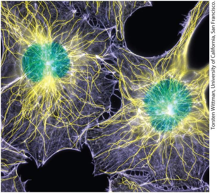
Chapter 4 Culturing and Visualizing Cells Fluorescence microscopy showing the locations of DNA (green), microtubules (yellow), and microfilaments (purple) in two cultured cells. The cells were chemically fixed and then rendered permeable to antibodies using a gentle detergent. Microtubules were stained with an antibody to tubulin; microfilaments were stained with a labeled toxin, phalloidin, that binds selectively to F-actin; and DNA was visualized with a DNA-binding dye.

4.2 Light Microscopy: Exploring Cell Structure and Visualizing Proteins Within Cells

4.4 Isolation of Cell Organelles It is difficult to believe that just 200 years ago it was not yet appreciated that all living things are made of cells. In 1655, Robert Hooke used a primitive microscope to examine a piece of cork and saw an orderly arrangement of rectangles — the walls of the dead plant cells — that reminded him of monks’ cells in a monastery, so he coined the term cell. Shortly after this, Antoni van Leeuwenhoek’s observations of the microorganisms he saw in his simple microscope became the first description of live cells. Two hundred years later, Matthias Schleiden and Theodore Schwann proposed that cells constitute the fundamental unit of life in plants, animals, and single-celled organisms. Collectively, these discoveries were some of the greatest in biology and posed the question of how cells are organized and function. Even today, many technical constraints hamper studies of cells in intact animals and plants. One alternative is the use of intact organs that are removed from animals and treated to maintain their physiological integrity and function. However, the organization of organs, even isolated ones, is sufficiently complex to pose numerous problems for research.

Thus molecular cell biologists often conduct experimental studies on cells isolated from an organism. In Section 4.1, we learn how to maintain and grow diverse cell types and how to isolate specific types of cells from complex mixtures. In many cases, isolated cells can be maintained in the laboratory under conditions that permit their survival and growth, a procedure known as culturing. Cultured cells have several advantages over intact organisms for cell biology research. Cells of a single specific type can be grown in culture, experimental conditions can be better controlled, and in many cases a single cell can be readily grown into a colony of many identical cells. The resulting strain of cells, which are genetically homogeneous, is called a clone. However, cultured cells are not in their native setting, so researchers are now growing and examining cells in three-dimensional environments to more closely mimic their situation in an animal. Discoveries about cellular organization have been intimately tied to developments in microscopy. This is as true today as it was 400 years ago. Light microscopy initially revealed the beautiful internal organization of cells, and today highly sophisticated microscopes are continually being improved to probe deeper and deeper into the molecular mechanisms by which cells function. In Section 4.2, we discuss light microscopy and the long-standing but still valuable techniques that are in use today, and then examine several clever methods that have been developed more recently, culminating with the newest, cutting-edge technologies. A major advance came in the 1960s and 1970s with the development of immunofluorescence microscopy, which allows the localization of specific

proteins within fixed cells, thus providing a static image of their location, as illustrated in the chapter-opening figure. Such studies led to the important understanding that the membranes and interior spaces of each type of organelle contain a distinctive group of proteins that are necessary for the organelle to carry out its unique functions. Another major advance came in the mid-1990s with the simple idea of expressing chimeric proteins — consisting of a protein of interest covalently linked to a naturally fluorescent protein — which has enabled biologists to visualize movements of individual proteins in live cells. Suddenly, the dynamic nature of cells could be appreciated. This has dramatically changed our view of cells when we were limited to only static images. Microscopes with higher sensitivity coupled with methods to enhance resolution now allow investigators to gain more information about the detailed structure and dynamics of cells. The development of fluorescence techniques also led to the development of methods to monitor protein-protein interactions in live cells, as well as a myriad of other sophisticated molecular technologies, some of which we discuss in this section. For decades, light microscopy was constrained by the resolution of the light microscope — to about 200 nm — due to the limitations imposed by the wavelength of visible light. We discuss methods that have been developed over the last few years to beat this resolution barrier with the development of superresolution microscopy. Despite the amazing developments in light microscopy, visible light still provides too low a resolution to examine cells in fine, ultrastructural detail. The electron microscope gives a much higher resolution, but the technology generally requires that the cell be fixed and sectioned, and

therefore all cell movements are frozen in time. Electron microscopy also allows investigators to examine the structure of macromolecular complexes or single macromolecules. In Section 4.3, we outline the various approaches for preparing specimens for observation in the electron microscope and describe the types of information that can be derived from them. Light and electron microscopy revealed that all eukaryotic cells contain a similar repertoire of membrane-limited compartments termed organelles. In parallel with the developments in microscopy, subcellular fractionation methods were developed that have enabled cell biologists to isolate individual organelles to a high degree of purity. These techniques, detailed in Section 4.4, continue to provide important information about the protein composition and biochemical function of organelles.

Culture of Animal Cells Requires Nutrient-Rich Media and Special Solid Surfaces

4.1 Growing and Studying Cells in Culture The study of cells is greatly facilitated by growing them in culture, so that they can be examined by microscopy and subjected to specific treatments under controlled conditions. It is generally quite easy to grow unicellular bacteria, fungi, or protists, for example, by placing them in a rich medium that supports their growth. However, animal cells come from multicellular organisms, which makes it more difficult to culture single cells or small groups of cells. In this section, we discuss how animal cells are grown in culture and how different cell types can be purified for study. Culture of Animal Cells Requires Nutrient-Rich Media and Special Solid Surfaces To permit the survival and normal function of cultured tissues or cells, the temperature, pH, ionic strength, and access to essential nutrients must simulate as closely as possible the conditions within an intact organism. Isolated animal cells are typically placed in a nutrient-rich liquid, called the culture medium, within specially coated plastic dishes or flasks. The cultures are kept in incubators in which the temperature, atmosphere, and humidity can be controlled. To reduce the chances of bacterial or fungal

contamination, antibiotics are often added to the culture medium. To further guard against contamination, investigators usually transfer cells between dishes, add reagents to the culture medium, and otherwise manipulate the specimens within special sterile cabinets containing circulating air that is filtered to remove microorganisms and other airborne contaminants. Media for culturing animal cells must supply the nine amino acids (phenylalanine, valine, threonine, tryptophan, isoleucine, methionine, leucine, lysine, and histidine) that cannot be synthesized by adult vertebrate animal cells. In addition, most cultured cells require three other amino acids (cysteine, tyrosine, and arginine) that are synthesized only by specialized cells in intact animals, as well as glutamine, which serves as a nitrogen source. The other necessary components of a medium for culturing animal cells are vitamins, various salts, fatty acids, glucose, and serum — the fluid remaining after the noncellular part of blood (plasma) has been allowed to clot. Serum contains various protein factors that are needed for the proliferation of mammalian cells in culture, including the polypeptide hormone insulin; transferrin, which supplies iron in a bioaccessible form; and numerous growth factors. In addition, certain cell types require specialized protein growth factors not present in serum. For instance, progenitors of red blood cells require erythropoietin, and T lymphocytes require interleukin 2 (see Chapter 16). A few mammalian cell types can be grown in a chemically defined, serum-free medium containing amino acids, glucose, vitamins, and salts plus certain trace minerals, specific protein growth factors, and other components.

Primary Cell Cultures and Cell Strains Have a Finite Life Span

Unlike bacterial and yeast cells, which can be grown in suspension, most animal cell types will grow only when attached to a solid surface. This requirement highlights the importance of the cell-surface proteins, called cell-adhesion molecules (CAMs), that cells use to bind to adjacent cells and to components of the extracellular matrix such as collagen, laminin, or fibronectin (see Chapter 20). The solid growth surface (usually glass or plastic) is either pre-coated with these extracellular-matrix proteins, or they come from the serum or are secreted by the cells in culture. A single cell cultured on a glass or plastic dish proliferates to form a visible mass, or colony, containing thousands of genetically identical cells in 4 to 14 days, depending on the growth rate. Although most normal animal cells require a surface to grow on, some specialized blood cells, and especially tumor cells, can be grown in suspension as single cells. Primary Cell Cultures and Cell Strains Have a Finite Life Span Primary cells are cells isolated directly from tissues. Normal animal tissues (e.g., skin, kidney, liver) or whole embryos are commonly used to establish primary cell cultures. To prepare individual tissue cells for a primary culture, the cell-cell and cell-matrix interactions must be broken. To do so, tissue fragments are treated with a combination of a protease (e.g., trypsin, the collagen-hydrolyzing enzyme collagenase, or both) and a divalent cation chelator (e.g., EDTA) that depletes the medium of free calcium . Many CAMs require calcium and are thus inactivated when calcium is removed; other CAMs that are not calcium dependent

need to be cleaved by a protease for the cells to separate. The released cells are then placed in a nutrient-rich, serum-supplemented medium in dishes, where they can adhere to the surface and to one another. The same protease-chelator solution is used to remove adherent cells from a culture dish for biochemical studies or subculturing (transfer to another dish). Fibroblasts are the predominant cells in connective tissue and normally produce extracellular-matrix components, such as collagen, that bind to CAMs, thereby anchoring cells to a surface. In culture, fibroblasts usually divide more rapidly than other cells from a tissue, eventually becoming the predominant cell type in a primary culture unless special precautions are taken to remove them when isolating other types of cells. When cells removed from an embryo or an adult animal are cultured, most of the adherent cells will divide a finite number of times and then cease growing (a phenomenon called cell senescence). For instance, human fetal fibroblasts divide about 50 times before they cease growth. Starting with cells, 50 doublings has the potential to produce , or more than , cells, whose weight would be equivalent to that of about a thousand people. Normally, only a very small fraction of these cells are used in any one experiment. Thus even though its lifetime is limited, a single culture, if carefully maintained, can be studied through many cell generations. Such a lineage of cells originating from one initial primary culture is called a cell strain. One important exception to the finite life span of normal cells is the embryonic stem cell, which, as its name implies, is derived from an

Transformed Cells Can Grow Indefinitely in Culture

embryo and will divide and give rise to all tissues during development. As we discuss in Chapter 22, embryonic stem cells can be cultured indefinitely under the appropriate conditions. Research with cell strains is simplified by our ability to freeze them and successfully thaw them at a later time for experimental analysis. Cell strains can be frozen in a state of suspended animation and stored for extended periods at liquid nitrogen temperature, provided that a preservative that prevents the formation of damaging ice crystals is used. Although not all cells survive thawing, many do survive and resume growth. Transformed Cells Can Grow Indefinitely in Culture To be able to clone individual cells, modify cell behavior, or select mutants, biologists often want to maintain cell cultures for many more than 50 doublings. Such prolonged growth is exhibited by cells derived from some tumors. In addition, rare cells in a population of primary cells may undergo spontaneous oncogenic mutations, leading to oncogenic transformation (see Chapter 25). Such cells, said to be oncogenically transformed, or simply transformed, are able to grow indefinitely. A culture of cells with an indefinite life span is considered immortal and is called a cell line.

Flow Cytometry Separates Different Cell Types

The HeLa cell line, the first human cell line established, was originally obtained in 1952 from a malignant tumor (carcinoma) of the uterine cervix and is still used extensively today. The cells were obtained from Henrietta Lacks without her consent, which has raised ethical issues concerning ownership of biological materials. Many other human cell lines are derived from cancers, and biologists have rendered others immortal by transforming them to express oncogenes. Regardless of their source, cells in immortal lines often have chromosomes with abnormal DNA sequences. In addition, the number of chromosomes in such cells is usually greater than that in the normal cell from which they arose, and the chromosome number changes as the cells continue to divide in culture. A noteworthy exception is a human cell line of hematopoietic origin that is haploid for all chromosomes except chromosome 8. Since inactivation of one of the two copies of a gene in a diploid cell generally does not generate a phenotype, a line with a single copy of most genes is very useful for genetic analysis, making possible the types of genetic screens employed in model organisms (see Chapter 6). Cells with an abnormal number of chromosomes are said to be aneuploid. Flow Cytometry Separates Different Cell Types Some cell types differ sufficiently in density that they can be separated on the basis of this physical property. White blood cells (leukocytes) and red blood cells (erythrocytes), for instance, have very different densities

because erythrocytes have no nucleus; thus these cells can be separated by equilibrium density-gradient centrifugation (described in Section 4.4). Most cell types cannot be differentiated so easily, so other techniques, such as flow cytometry, must be used to separate them. To separate one type of cell from a complex mixture, it is necessary to have some way to mark and then sort out the desired cells. As we will see below, it is possible to mark cells by expressing a fluorescent protein in them, but if only a few cells in the population express the protein, how can we sort them from the nonfluorescent ones? The cells can be analyzed in a flow cytometer. This machine flows cells past a laser beam that measures the light that they scatter and the fluorescence that they emit; thus it can quantify the cells expressing the fluorescent protein in a mixture. A fluorescence-activated cell sorter (FACS), which is based on flow cytometry, can both analyze the cells and select the few fluorescent cells from thousands of others and sort them into a separate culture dish (Figure 4-1). To achieve this, the cells are mixed with a buffer and forced through a vibrating nozzle to generate tiny droplets. The concentration of cells is adjusted so that most of the droplets do not contain cells, and the ones that do contain only one. Just before the nozzle, the stream of cells passes through a laser beam so that the presence and size of a cell can be recorded from the scattered light using one detector, and the amount of fluorescent light emitted can be quantified using a second, fluorescent light detector. If a cell is present in a droplet, the droplet is given a negative electric charge as it emerges from the nozzle. The stream of droplets then passes through two plates that generate an electric field proportional to the fluorescence detected from the cell in the droplet. This field generates a

force that moves charged droplets out of the stream of uncharged droplets and into a collection tube. Since the amount of force applied is proportional to the fluorescence emitted by the cell in the droplet, cells with different levels of fluorescence can be collected. Having been sorted from other cells, the selected cells can be grown in culture.

FIGURE 4-1 A fluorescence-activated cell sorter (FACS) separates cells having different levels of fluorescence. Step 1 : A concentrated suspension of labeled cells is mixed with a buffer so that the cells pass single file through a laser light beam. Step 2 : Both the fluorescent light emitted and the light scattered by each cell are measured; from

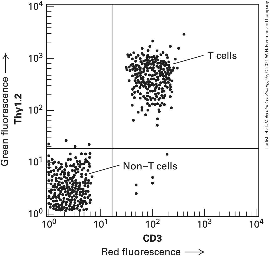
measurements of the scattered light, the size and shape of the cell can be determined. Step 3 : The suspension is then forced through a nozzle, which forms tiny droplets containing at most a single cell. At the time of formation at the nozzle tip, each droplet containing a cell is given a negative electric charge proportional to the fluorescence of that cell determined from the earlier measurement. Step 4 : Droplets now pass through an electric field, so that those with no charge are discarded, whereas those with different electric charges are separated and collected. Because it takes only milliseconds to sort each droplet, as many as 10 million cells per hour can pass through the machine. Description The illustration shows the suspension of cells surrounded by a sheath fluid passing through a nozzle. The fluorescent cells are represented in pink and light pink and the non-fluorescent cells in light blue. A laser beam is passed through the liquid containing fluorescent cells. Two detectors, oriented at right angles to each other, detect fluorescent light and scattered light. The cells emerging from the nozzle are separated by charged plates. The non-fluorescent light blue cells with no charge are discarded and the fluorescent pink and light pink cells with greater and lesser charges are separated in a glass beaker, respectively. The FACS procedure is commonly used to purify different types of white blood cells, each of which bears on its surface one or more distinctive proteins and so will bind monoclonal antibodies specific for its proteins. If a cell mixture is incubated with a fluorescent dye linked to the antibody to a specific cell-surface protein, only the desired cells will be fluorescent. Only the T cells of the immune system, for instance, have both CD3 and Thy1 proteins on their surfaces. The presence of these surface proteins allows T cells to be separated easily from other types of blood cells or spleen cells (Figure 4-2).

EXPERIMENTAL FIGURE 4-2 FACS separates T cells with bound fluorescence-tagged antibodies to two cell-surface proteins from other white blood cells. Spleen cells from a mouse were treated with a red fluorescent monoclonal antibody specific for the CD3 cellsurface protein and with a green fluorescent monoclonal antibody specific for a second cellsurface protein, Thy1. As the cells passed through a FACS, the intensity of the green and red fluorescence emitted by each cell was recorded. Each dot represents a single cell. This plot of green fluorescence (vertical axis) versus red fluorescence (horizontal axis) for thousands of spleen cells shows that about half of them — the T cells — express both CD3 and Thy1 proteins on their surfaces (upper-right quadrant). The remaining cells, which exhibit low fluorescence (lower-left quadrant), express only background levels of these proteins and are other types of white blood cells. Note the logarithmic scale on both axes.

[Data from Chengcheng Zhang, Whitehead Institute.] Description The vertical axis plots green fluorescence T h y 1.2 and ranges from 10 to the power 0 to 10 to the power 4 in increments of 10 to the power 1. The horizontal axis plots red fluorescence C D 3 and ranges from 10 to the power 0 to 10 to the power 4 in increments of 10 to the power 1. The plot is divided into four uneven quadrants with an intersection point 10 to the power 1 on both axes. Data points are represented by small dots in each quadrant. The data values are approximate. The upper-left quadrant near 10 to the power 1 contains four data points. The upper-right quadrant from 10 to the power 2 to 10 to the power 3 contains more than 200 data points and is labeled “T cells”. The lower-left quadrant contains more than 200 data points and is labeled “NonT cells”. The lower-right quadrant contains five data points. Flow cytometry can measure many different parameters in cells. For example, it can measure a cell’s DNA content (from the amount of fluorescence emitted from a DNA-binding dye) and determine the general shape and size of a cell (from the amount of scattered light). Measurements of the DNA content of individual cells are used to follow replication of DNA as cells progress through the cell cycle (see Chapter 19). Flow cytometry can also be used to identify specific cell types in a population by using cell-type specific antibodies, each with a different fluorescent molecule attached. An example is distinguishing different cell types in blood samples. It can also be used to study signaling pathways at the single-cell level. Stimulation of many signaling pathways results in the phosphorylation of specific proteins (discussed in Chapters 15 and 16), and these can often be detected in cell populations by western blot analysis using phospho-specific antibodies that recognize individual sites of phosphorylation on specific proteins (see Chapter 3). However, this yields

Growth of Cells in Two-Dimensional and Three-Dimensional Culture Mimics the In Vivo Environment

a population average, so flow cytometry has been adapted to quantify the phosphorylation level of specific proteins in individual cells. Use is made of phospho-specific antibodies to which different fluorescent reporters have been covalently linked. For example one antibody might be linked to a fluorochrome that emits green fluorescence, and another antibody linked to one that emits red fluorescence. Cells are treated so that they are made permeable to antibodies, but their phosphorylated proteins are retained. The permeabilized cells are then incubated with phospho-specific antibodies and analyzed by flow cytometry to detect the degree of phosphorylation of the proteins, as reported by the amount of green or red signal. In this way, the level of protein phosphorylation can be assessed in response to activation of different signaling pathways. An alternative method for separating specific types of cells uses small magnetic beads coupled to antibodies to a specific cell-surface molecule. For example, to isolate T cells, the beads are coated with a monoclonal antibody specific for a surface protein such as CD3 or Thy1. Only cells with these proteins will stick to the beads, which can be recovered from the preparation by attraction to a small magnet on the side of a test tube. Growth of Cells in Two-Dimensional and Three-Dimensional Culture Mimics the In Vivo Environment While much has been learned using cells grown on plastic or glass surfaces, these surfaces are far removed from cells’ normal tissue

environment. As detailed in Chapter 20, many cell types function only when closely linked to other cells. Key examples are the sheet-like layers of epithelial tissue, called epithelia (singular, epithelium), that cover the external and internal surfaces of organs. Typically, epithelial cells have distinct surfaces, called the apical (top), basal (base or bottom), and lateral (side) surfaces (see Figure 20-11). The basal surface usually contacts an underlying extracellular matrix called the basal lamina, whose composition and function are discussed in Section 20.3. Epithelial cells often function to transport specific classes of molecules across the epithelial sheet; for example, the epithelial lining of the intestine transports nutrients into the cell through the apical surface and out toward the bloodstream across the basolateral surface. When grown on plastic or glass, epithelial cells cannot easily perform this function. Therefore, special containers have been designed with a porous surface that acts as a basal lamina to which epithelial cells attach and form a uniform twodimensional sheet (Figure 4-3). A commonly used cultured cell line derived from dog kidney epithelium, called the Madin-Darby canine kidney (MDCK) cell line, is often used to study the formation and function of epithelial sheets.

FIGURE 4-3 Madin-Darby canine kidney (MDCK) cells grown in specialized containers provide a useful experimental system for studying epithelial cells. MDCK cells form a polarized epithelium when grown on a porous membrane filter coated on one side with collagen and other components of the basal lamina. With the use of the special culture dish shown here, the medium on each side of the filter (apical and basal sides of the monolayer) can be experimentally manipulated and the movement of molecules across the layer monitored. Description The illustration shows a cross-section of a round, clear culture dish containing a smaller inner chamber, which is also circular and roughly nine-tenths of the size of the culture dish. The space between the inner chamber and outer walls of the culture dish forms an outer chamber that contains a basal medium. A porous filter horizontally divides the inner chamber into two sub-compartments. The top sub-compartment is filled with apical medium and the bottom sub-compartment is filled with basal medium. Small holes at the bottom of the lower sub-compartment allow the free transfer of basal medium to the outer chamber. The dividing porous filter supports the basal lamina, which, in turn, supports a monolayer of M D C K cells. Each M D C K cell is depicted as a small square containing a single nucleus. The top side of the M D C K cell monolayer contains cilia in contact with the apical medium in the upper subcompartment, labeled “apical surface”. The bottom side of the M D C K cell monolayer

is in contact with the basal lamina, labeled “basal surface”. The sides of the M D C K cells in contact with each other and/or with the walls of the inner chamber are labeled "lateral surface". However, even a two-dimensional sheet often does not allow cells to fully mimic behavior in their normal environment. Methods have now been developed to grow cells in three dimensions by providing a support infiltrated with appropriate components of the extracellular matrix (discussed in Chapter 20). If MDCK cells are cultured under appropriate conditions, they will form a tubular sheet mimicking a tubular organ or the duct of a secretory gland. In these three-dimensional structures, the apical side of the epithelial sheet lines the lumen, whereas the basal side of each cell is in contact with the extracellular matrix (Figure 4-4). EXPERIMENTAL FIGURE 4-4 MDCK cells can form cysts in culture. (a) MDCK cells grown on a supported extracellular matrix will form groups of cells that polarize to form a tubular single layer of cells with a lumen in the middle, called a cyst. (b) By examining the localization of proteins found in the apical (red) and basolateral membranes (green), we can

Stem Cells Can Differentiate in Culture to Make Organoids

see that these cells are fully polarized, with the apical side facing the lumen, which recapitulates their organization in the kidney tubules from which they are derived. The nuclear DNA is stained blue. Description Micrograph labeled A shows M D C K cells in three-dimensional cell culture forming a cyst. The cyst in a spherical form with an uneven surface has smaller entities with various shapes. The fluorescent micrograph labeled B shows the stained spherical cyst. The cyst contains one circular section at its center, highlighted by staining for the apical membrane. The circular center is surrounded by six distinct sub-compartments, formed by basolateral membranes. Each of the six sub-compartments contains nuclear D N A, stained blue. The absence of staining in the central circle suggests that the apical membrane does not contain nuclear D N A. In a similar manner, primary hepatocytes (cells isolated from a liver) can now be isolated and cultured. Under proper conditions, they will form hepatocyte spheroids that can be maintained in culture and respond to drugs in much the same way that an intact liver does in living animals. These are just two examples of a growing field in which organ culture systems are being developed to more closely correspond to cells and tissues in living animals — and thereby expand the number of experiments that can be performed in a physiologically relevant manner. Stem Cells Can Differentiate in Culture to Make Organoids As we discuss in detail in Chapter 22, embryonic stem cells can be isolated from the inner cell mass of an early mammalian embryo. These

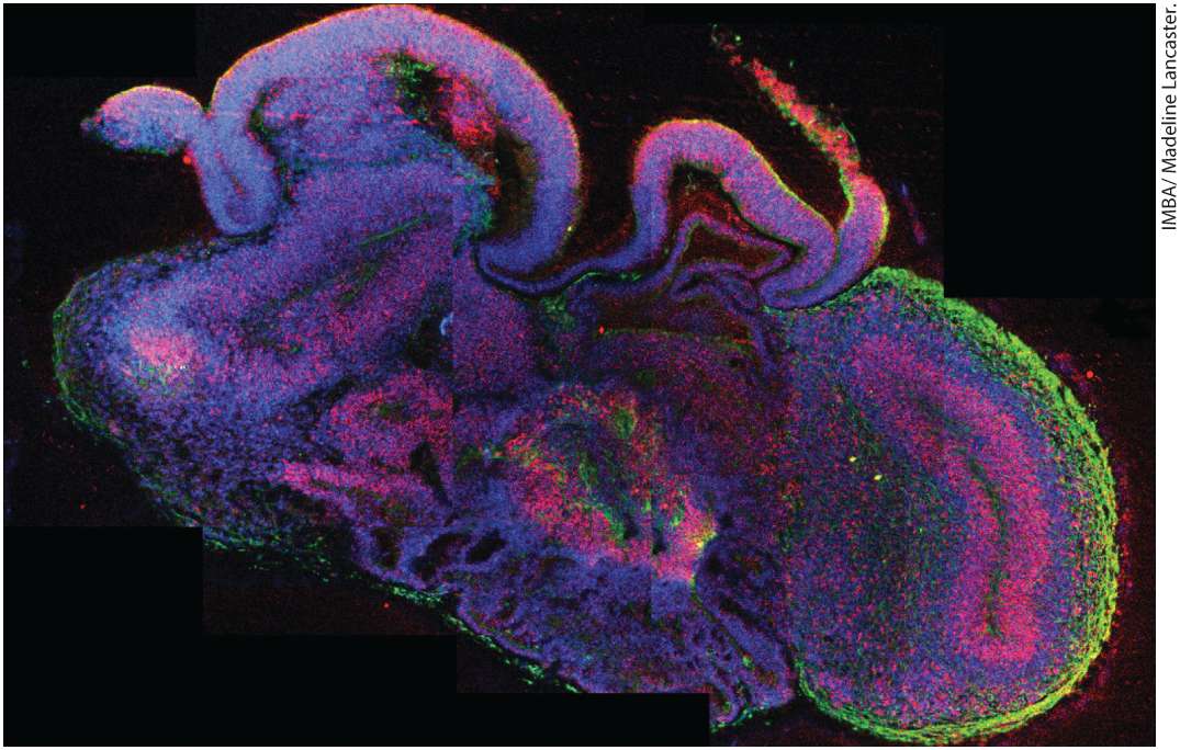
cells are pluripotent, that is, they can give rise to all tissues of the embryo. Mature animals have adult stem cells in their tissues. These cells are not pluripotent, but are nevertheless crucial for cell regeneration or tissue repair. The division and differentiation of cells in an animal is orchestrated by many factors, including interactions with the extracellular matrix and other cells, response to soluble factors, and temporal changes in gene expression. With major advances in the study of the extracellular matrix (discussed in Chapter 20), signaling pathways elucidated by developmental studies (see Chapters 15 and 16), and the regulation of gene expression (discussed in Chapter 8), much has been learned about the molecular details of these differentiation pathways. It is now possible to recapitulate some of these developmental events in culture. When adult stem cells from the intestine were placed in culture under appropriate conditions in a three-dimensional matrix, the cells formed intestinal organoids that had the normal crypt and villous structures of the small intestine. In a dramatic advance, researchers have used human pluripotent cells in culture to generate brain organoids whose organization and structure is remarkably similar to the fetal brain (Figure 4-5). Organoids have now been developed for many organs, including the brain, intestines, stomach, kidney, heart, and tongue. So far, organoids advance to a stage of development characterized in the fetus, but do not proceed to the organization seen in an adult organ. These astonishing results reveal that cells possess the intrinsic program to divide, differentiate, and organize themselves into complex structures.

EXPERIMENTAL FIGURE 4-5 Brain organoid derived from pluripotent stem cells. In this section of the organoid, neural stem cells are labeled red and neurons are green. All cell nuclei are stained blue. Description The left edges of the brain organoid are mostly blue. The organoid center is mostly a blend of blue and red. The right edges of the organoid are enveloped in a layer of green. Blue stains represent cell nuclei, the red stains represent neural stem cells, and the green stains represent neurons. Besides being a remarkable achievement, what uses can be made of organoids? First, cells in an organoid can be followed much more easily than in a living animal. For example, in brain organoids, it will be possible to examine early human brain development in much more detail. Second, stem cells used to generate organoids can be manipulated by introducing

mutations and then observed to see how they affect the development of the organoid. Third, it is possible to test the effects of drugs on organoid development, which is much easier than in animals. Fourth, it has been found that tumor cells removed from a patient can be used to generate a morphologically characteristic tumor organoid in culture — which can be used to test the efficacy of potential drugs before they are administered to a patient. These are just a few of the remarkable uses for organoids; many more creative uses for both basic science and medicine are being developed. Can we grow a whole organ that could be transplanted into a patient? As indicated above, organoids grown in culture so far do not develop into adult organs. However, recent advances in biomedical engineering are developing promising strategies to do this, initially in experimental animals. In an example of one approach, a 3-D printer is used to help make a replacement ear. First, an exact computer image of an ear is generated. This image is used to program a 3-D printer to assemble a pliable matrix — containing support material that is biodegradable, together with appropriate components of the extracellular matrix — in the precise shape of an ear. This matrix provides support for the growth of skin cells, either in culture or after transplantation under the skin, so that ultimately the synthetic organ can be surgically attached to a living animal. Other approaches make use of 3-D printers to assemble the matrix and seed it with appropriate cells. An exciting and ambitious goal of this technology is to generate synthetic organs containing many different types of cells by printing each of several layers with the appropriate matrix and

Hybridomas Produce Abundant Monoclonal Antibodies

cells to generate complex three-dimensional organs that might one day be used to replace defective ones in patients. Many hurdles still need to be overcome, but the ability to generate stem cells from patients and then induce differentiation in culture is overcoming the major obstacle of immunological rejection and will probably be key to providing cells for the assembly of synthetic organs. Hybridomas Produce Abundant Monoclonal Antibodies In addition to serving as research models for studies of cell function, cultured cells can be converted into “factories” for producing specific proteins. For example, special cultured cells can be used to generate monoclonal antibodies, which are experimental tools widely used in many aspects of cell biological research. They are also used for diagnostic and therapeutic purposes in medicine, as we discuss in later chapters. To understand the challenge of generating monoclonal antibodies, we must briefly review how mammals produce antibodies; more detail is provided in Chapter 24. Recall that antibodies are proteins secreted by white blood cells that bind with high affinity to their antigen (see Figure 3-22). Each normal antibody-producing B lymphocyte in a mammal is capable of producing a single type of antibody that can bind to a particular determinant, or epitope, on an antigen molecule. An epitope is generally a small region on the antigen, consisting, for example, of just a few amino acids. If an animal is injected with an antigen, the B lymphocytes that

make antibodies recognizing that antigen are stimulated to grow and secrete those antibodies. Each antigen-activated B lymphocyte forms a clone of cells in the spleen or lymph nodes, with each cell producing the identical antibody — that is, a monoclonal antibody. Because most natural antigens contain multiple epitopes, exposure of an animal to an antigen usually stimulates the formation of multiple B-lymphocyte clones, each producing a different antibody. The resulting mixture of antibodies from the many B-lymphocyte clones that recognize different epitopes on the antigen is said to be polyclonal. Such polyclonal antibodies circulate in the blood and can be isolated as a group. Although polyclonal antibodies are very useful, monoclonal antibodies are more suitable for many types of experiments and medical applications in which we need a reagent that binds to just one site on a protein; for example, one that competes with a ligand on a cell-surface receptor. Unfortunately, the biochemical purification of any one type of monoclonal antibody from blood is not feasible for two main reasons: the concentration of any given antibody is quite low, and all antibodies have the same basic molecular architecture (see Figure 3-22). To produce and then purify monoclonal antibodies, one first needs to be able to grow the appropriate B-lymphocyte clone. However, primary cultures of normal B lymphocytes are of limited usefulness for the production of monoclonal antibodies because they have a limited life span. Thus the first step in producing a monoclonal antibody is to generate a library of immortal antibody-producing cells (Figure 4-6). Immortality is achieved by fusing normal B lymphocytes from an immunized animal

with transformed, immortal lymphocytes called myeloma cells that themselves do not synthesize antibodies, and selecting for hybrid cells called a hybridoma. Like myeloma cells, hybridoma cells grow rapidly and are immortal. Each hybridoma produces the monoclonal antibody encoded by its B-lymphocyte parent. The library of hybridomas is then screened for clones that produce the desired antibody; any clone producing that antibody is then grown in large cultures, from which a substantial quantity of pure monoclonal antibody can be obtained.

FIGURE 4-6 Use of cell fusion and selection to obtain hybridomas producing a monoclonal antibody to a specific protein. Step 1 : Immortal myeloma cells that cannot synthesize purines under special conditions because they lack thymidine kinase are fused with normal antibody-producing spleen cells from an animal that was immunized with antigen X. Step 2 : When cultured in a special selective medium, unfused and self-fused cells do not grow: the myeloma cells do not grow because the selective medium does not contain purines, and the spleen cells do not grow because they have a limited life span in culture. Thus only fused cells formed from a myeloma cell and a spleen cell survive in the selective medium, proliferating into clones called hybridomas. Each hybridoma produces a single antibody. Step 3 : Testing of individual clones identifies those that recognize antigen X. After a hybridoma that produces a desired antibody has been identified, the clone can be cultured to yield large amounts of that antibody. Description The flowchart shows a cartoon of a mouse injected with antigen X and its spleen cells are subsequently harvested. The spleen cells are depicted as small red and blue circles and a small fraction of them are labeled as “Mouse spleen cells; some cells (red) make an antibody to antigen X.” In step one, all isolated mouse spleen cells are mixed and fused with mutant mouse myeloma cells (yellow circles) that are unable to grow in selective medium. At this step, both anti-X antibody-producing (red) and non-anti-X antibody-producing (blue) spleen cells are fused with myeloma cells (yellow). In step two, the cell mixture is transferred to a round cell culture dish containing selective medium. Once cultured, only fused cells (orange and green) can survive and grow in the selective medium. In step three, each surviving cell is transferred to a separate well in a new culture dish. Each well is subsequently tested for the presence of antibody against antigen X. Monoclonal antibodies are valuable research tools. They are commonly employed in affinity chromatography to isolate and purify proteins from complex mixtures (see Figure 3-43c). As we discuss later in this chapter, they are also employed in immunofluorescence microscopy to locate a

particular protein within cells, and they are used in immunoblotting to identify specific proteins in cell fractions (see Figure 3-44). Rabbit, mouse, and human immunoglobulins are built from two heavy chains and two light chains, with both the light and heavy chains contributing to the antigen binding site (see Figure 24-14). Remarkably, camelids (including camels and llamas) have these conventional immunoglobulins and immunoglobulins consisting of just two heavy chains. The antigen-combining site of these antibodies is relatively small, about 15 kDa compared with about 150 kDa for a whole mouse monoclonal antibody. Thus the camelid immunoglobulins are easily expressed in, and purified from, bacteria. Such so-called nanobodies with a single high-affinity binding site for specific antigens are being developed for therapeutic, diagnostic, and research purposes. Monoclonal antibodies have become important diagnostic and therapeutic tools in medicine as well. For example, monoclonal antibodies that bind to and inactivate toxins secreted by bacterial pathogens are used to treat certain infectious diseases. The first monoclonal antibodies used for therapeutic purposes were made in mice. However, when used in humans these were recognized as foreign proteins and removed by the immune system. Subsequently, antibodies were engineered to contain mostly human sequences fused to the mouse antigen-binding regions. An early example of such a therapeutic antibody was the development of Herceptin for treatment of an aggressive form of

A Wide Variety of Cell Biological Processes Can Be Studied with Cultured Cells

breast cancer. It was known that these cancers overexpress HER2, a plasma membrane protein of the EGF receptor tyrosine kinase family (see Chapter 16). Monoclonal antibodies to the extracellular domain of HER2 were generated and screened for those that reduced HER2-overexpressing tumors in mice. Refining and humanizing this mouse monoclonal antibody resulted in the development of Herceptin, which has now been used to treat about a half million patients with HER2-positive breast cancer. Therapeutic antibodies are available today with about 85–90 percent human sequences, although generating these is a technologically complicated process. A much better solution would be to generate monoclonal antibodies directly from human B cells. Recently, such an approach has been made possible. To make human monoclonal antibodies, many millions of naive B cells are isolated from removed tonsils. Since the isolated cells cannot be propagated indefinitely, the population is immortalized by infecting them with Epstein-Barr virus. The immortal naive B cells are induced to undergo class-switching and somatic mutations (discussed in Chapter 24) to generate an extensive library of B cells in which each clone secretes a specific monoclonal antibody. The library of B cells can then be screened with antigen for those that secrete the desired monoclonal antibody. In this way, it will be possible to isolate human-based therapeutic monoclonal antibodies.

A Wide Variety of Cell Biological Processes Can Be Studied with Cultured Cells As we discussed in the introduction to this chapter, studying animal cells in culture is much easier than studying cells in intact animals, partly because they can easily be subjected to a variety of manipulations. Cultured cells are particularly useful for the elucidation of fundamental processes. One way to understand a biological process is to interfere with a specific constituent in the cell and assess the outcome — this approach is like trying to understand how a car works by removing components and seeing what goes wrong. In some cases, human diseases associated with genetic defects in specific cell components can be analyzed using cells cultured from the patients. For example, analysis of cultured cells from patients with a genetic defect resulting in hypercholesterolemia — who have elevated blood cholesterol leading to heart disease and stroke — was critical in elucidating the basic steps of receptor-mediated endocytosis (see Chapter 14). In addition to relying on naturally occurring genetic lesions, we can manipulate cultured cells to interfere with expression of specific components. As we will see in Chapter 6, it is possible to decrease the expression of a specific protein in cultured cells by selectively knocking down the corresponding mRNA and then assess what effect this change has on particular processes in the cell. Chapter 6 also describes the more recently developed gene editing techniques that can be used to inactivate specific genes in the genomes of cultured cells and thereby

Drugs Are Commonly Used in Cell Biological Research

assess how the complete loss of specific RNAs and proteins affects cell functions. Drugs Are Commonly Used in Cell Biological Research Another powerful way to analyze biological processes is to treat cells with drugs that bind to specific cell components and inactivate or activate them. In this section, we discuss how new drugs affecting specific cell processes can be developed. Naturally occurring drugs have been used for centuries, but how they worked was often unknown. For example, extracts of meadow saffron were used to treat gout, a painful disease resulting from inflammation of joints. Today we know that this plant contains colchicine, a drug that depolymerizes microtubules (see Chapter 18) and interferes with the ability of white blood cells to move to sites of inflammation. Alexander Fleming discovered that certain fungi secrete compounds that kill bacteria (antibiotics), and his discovery resulted in the development of penicillin. Only later was it discovered that penicillin inhibits cell division by blocking the assembly of the cell walls of certain bacteria. Discoveries like these have resulted in a wide range of drugs that can inhibit specific and essential processes of cells. In most cases, researchers have eventually been able to identify the molecular targets of these drugs.

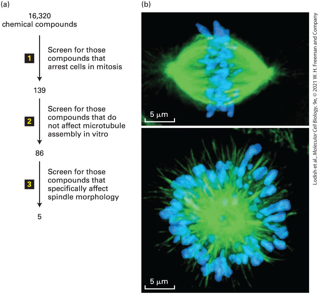
For example, there are many antibiotic drugs that affect aspects of prokaryotic protein synthesis. How does one discover a new drug? One widely used approach is to search chemical libraries, consisting of tens to hundreds of thousands of different compounds, for chemicals that inhibit a specific process. The screening of chemical libraries in conjunction with high-throughput microscopic techniques has now become one of the major routes for new leads in drug discovery. Here we give just one case to illustrate how this type of approach works. In our example (Figure 4-7a), researchers wanted to identify compounds that inhibit mitosis, the process by which duplicated chromosomes are accurately segregated by a microtubule-based machine called the mitotic spindle (discussed in Chapter 18). It was known that if spindle assembly is compromised, cells are arrested in mitosis. Therefore, the screen first used an automated robotic method to look for compounds that arrest cells in mitosis. The basis for the inhibition of mitosis by the candidate compounds was then explored to see if they affected assembly of the microtubules. Since inhibition of microtubule assembly was not of interest, the effect of the remaining candidate compounds on the structure of the spindle was determined by immunofluorescence microscopy using antibodies to tubulin, the major protein of microtubules. Over 16,000 compounds were screened, and a compound was identified that resulted in cells with abnormal spindles — instead of having two asters, they had a single aster, resulting in what is called a mono-astral array (Figure 4-7b). This drug, now called monastrol, was found to interfere with the assembly

of the spindle by inhibiting a microtubule-based motor protein called kinesin-5. (See Chapter 18 for more details about the mitotic spindle.) While monastrol did not have the appropriate properties for a clinically useful drug, other kinesin-5 inhibitors have been developed that are now in clinical trials.

FIGURE 4-7 Screening for drugs that affect specific biological processes. (a) In this example, a chemical library of 16,320 different chemicals was subjected to a series of screens for inhibitors of mitosis. Since such an inhibitor is expected to arrest cells at the mitotic stage of the cell cycle, the first screen (step 1 ) was to see if any of the chemicals

enhanced the level of a marker specific for mitotic cells; this screen yielded 139 candidates. Microtubules make up the structure of the mitotic spindle, and the researchers were not interested in new drugs that target microtubules, so in the second screen (step 2 ) they tested the 139 compounds for their ability to affect microtubule assembly; this test eliminated 53 candidates. Immunofluorescence microscopy with antibodies to tubulin (the major subunit of microtubules), together with a stain for DNA, was then used in the third screen (step 3 ) to identify compounds that disrupt the structure of the spindle. (b) Localization of tubulin (green) and DNA (blue) for an untreated mitotic spindle (top) and one treated with one of the five compounds remaining after screen, now called monastrol. Monastrol inhibits a microtubule-based motor protein called kinesin-5, discussed in Chapter 18, that is necessary to separate the poles of the mitotic spindle. When kinesin-5 is inhibited, the two poles remain associated to give a monopolar spindle. [Part (b) Republished with permission of American Association for the Advancement of Science from Mayer, T.U. et al., “Small molecule inhibitor of mitotic spindle bipolarity identified in a phenotype-based screen,” 1999, Science 286:971–974; permission conveyed through Copyright Clearance Center, Inc.] Description A flowchart labeled A shows the screening process in three steps. In the first step, a chemical library of 16,320 compounds is screened and 139 compounds are identified for their capacity to arrest cell in mitosis. In step two, the selected 139 compounds are further screened for those compounds that do not affect microtubule assembly in vitro. This second screen leads to the identification of 86 compounds from 139. In step three, the 86 compounds identified are further screened for compounds that specifically affect spindle morphology. The final point in the flow chart shows that the third screening step narrowed the list of compounds down to five candidates. The scale bar on both the micrographs read 5 micrometers. The first immunofluorescence micrograph shows a cell undergoing mitosis in the absence of inhibitor. The round cell appears to be stretched horizontally to form an oval. Tubulin staining shows the presence of tubulin proteins (green) throughout the cell interior. Chromosomal D N A (blue) is stained as distinct amorphous entities in the center of the cell, forming a vertical line dividing the oval cell in two. The second immunofluorescence micrograph shows a cell undergoing mitosis in the presence of monastrol, an inhibitor of mitotic spindle formation. The cell remains round in the presence of inhibitor and D N A staining reveals that

chromosomal D N A (blue) is not localized to the center of the cell, but is present in a circle around the inside edges of the cell. Tubulin proteins (green) are present throughout the surface of the cell. KEY CONCEPTS OF SECTION 4.1 Growing and Studying Cells in Culture Animal cells have to be grown in culture under conditions that mimic their natural environment, which generally requires them to be supplied with necessary amino acids and growth factors. Most animal cells need to adhere to a solid surface to grow. Primary cells — those isolated directly from tissue — have a finite life span. Transformed cells, such as cells derived from tumors, can grow indefinitely in culture. Cells that can be grown indefinitely are called a cell line. Many cells lines are aneuploid, having a different number of chromosomes than the parent cell from which they were derived. Cells expressing a fluorescent protein can be sorted on a machine called a fluorescence-activated cell sorter (FACS) (see Figure 4-2). Different cell types express different marker proteins on their cell surfaces, which can be labeled with fluorescent markers, allowing them to be sorted on a FACS machine. Epithelial cells are often grown in special containers to mimic their functional polarity. Cells can also be grown on three-dimensional matrices to more accurately reflect their normal environment. Monoclonal antibodies, which bind one epitope on an antigen, can be secreted by cultured cells called hybridomas. These hybrid cells are made by fusing antibodyproducing B lymphocytes with immortal myeloma cells and then identifying those clones that produce the desired antibody. Monoclonal antibodies are important for basic research and as therapeutic agents (see Figure 4.6). Cells in culture can be much more easily manipulated than cells in an intact animal. Basic biological processes can be studied by interfering with specific cell components, either through genetic mechanisms or by the application of specific drugs. Large chemical libraries can be screened for compounds that target specific processes to study those processes and to identify new drugs.

4.2 Light Microscopy: Exploring Cell Structure and Visualizing Proteins Within Cells

4.2 Light Microscopy: Exploring Cell Structure and Visualizing Proteins Within Cells The cellular basis of life was first appreciated using primitive light microscopes. Since then, progress in cell biology has paralleled, and has often been driven by, technological advances in light microscopy (Figure 4-8). Here we discuss each of these major developments and how they advanced the study of cellular processes. First we describe basic uses of a light microscope to observe unstained cells and structures, or material treated with chemical stains. Next we describe how fluorescence microscopy is used to localize specific proteins in fixed cells. By using molecular genetic techniques to fuse a protein of interest with a naturally fluorescent protein and express the resulting chimeric protein in cells, it is possible to follow the movement of specific proteins in live cells — an ability that has revealed the dynamic organization of live cells. In parallel with these advances in specimen preparation, optical advances were being made that enhance and sharpen the images provided by fluorescence microscopy, revealing cellular structure with unprecedented resolution. Many specialized technologies have emerged from these advances, and we describe some of the more important ones.

FIGURE 4-8 Development of the light microscope. (a) Early microscopes, like the ones used by Robert Hooke in the 1660s, used lenses or a mirror to illuminate the specimen. (b) Optics in general, and light microscopes in particular, developed enormously during the nineteenth century. By the middle of the twentieth century, highly sophisticated microscopes limited only by the resolution of light were common. (c) In the second half of the twentieth century, fluorescence microscopy and digital imaging, together with confocal techniques, were developed to yield the versatile microscopes of today. Description The photo labeled A shows an early microscope model. This model consists of a mounted metallic cylinder with the objective pointing down toward a wooden mounting stage. Next to the microscope are two glass balls mounted to direct light toward the mounting stage. One glass ball has a spherical shape and the other is oval. The photo labeled B shows a modern microscope. This model is made primarily of hard plastic and metal. It is visually more sophisticated than the early microscope. The photo labeled C shows a large modern microscope attached to a desktop computer for digital imaging. To the left of the microscope is the desktop computer that displays a fluorescent microscopy image of immunostained cells. Many of the microscopy techniques we discuss allow one to examine live cells. These include live cell imaging as well as examining responses of live cells to a specific stimulus, such as a growth factor, or their interactions with other cells. These techniques have provided scientists

The Resolution of the Conventional Light Microscope Is About 0.2 μm

with the ability to probe the functioning of individual components in live cells. The Resolution of the Conventional Light Microscope Is About All microscopes produce a magnified image of a small object, but the nature of the image depends on the type of microscope employed and on the way the specimen is prepared. The compound microscope, used in conventional bright-field light microscopy, contains several lenses that magnify the image of a specimen under study (Figure 4-9a, b). The total magnification is a product of the magnification of the individual lenses: if the objective lens, the lens closest to the specimen, magnifies hundredfold (a , the maximum usually employed), and the projection lens that focuses the image on a camera magnifies tenfold, the final magnification will be 1000-fold. Alternatively, if the light is directed to an ocular or eyepiece lens that magnifies tenfold, the final magnification recorded by the human eye will also be 1000-fold.

FIGURE 4-9 Optical microscopes are commonly configured for bright-field, phasecontrast, or fluorescence microscopy. (a) In a typical light microscope, the specimen is usually mounted on a transparent glass slide and positioned on the movable specimen stage.

(b) In bright-field light microscopy, light from a tungsten lamp is focused on the specimen by a condenser lens below the stage; the light travels the pathway shown in yellow. (c) In phase-contrast microscopy, incident light passes through an annular diaphragm, which focuses a circular annulus (ring) of light on the specimen. Light that passes unobstructed through the specimen is focused by the objective lens onto the thicker gray ring of the phase plate, which absorbs some of the direct light and alters its phase by one-quarter of a wavelength. If a specimen refracts (bends) or diffracts the light, the phase of some light waves is altered (green lines), and the light waves pass through the clear region of the phase plate. The refracted and unrefracted light is recombined at the image plane to form the image. (d) In fluorescence microscopy, a beam of light from a mercury lamp (gray lines) is directed to the excitation filter, which allows only the correct wavelength of light to pass through (green lines). The light is then reflected off a dichroic mirror and through the objective lens, which focuses it on the specimen. The fluorescent light emitted by the specimen (red lines) passes up through the objective lens, then through the dichroic mirror, and is focused and recorded on the detector at the image plane. Description The illustration labeled A shows the components of the light microscope. The components of the light microscope are as follows: Detector, projection lens, dichroic mirror, objective, specimen stage, condenser, mirror, collector lens, lamps, and excitation filter. An oval inset shows an enlargement of the objective, including the lens angle. The illustration labeled B shows the components of the bright-field microscope. The components of the bright-field microscope are as follows: Projection lens, objective lens, specimen, condenser lens, mirror, and light source. The illustration labeled C shows the components of the phase-contrast microscope. The components of the phase-contrast microscope are as follows: Projection lens, phase plate in the objective, objective lens, specimen, annular diaphragm, mirror, and light source. The illustration labeled D shows the components of the fluorescence microscope. The components of the fluorescence microscope are as follows: Image plane, projection lens, dichroic mirror, objective lens, specimen, excitation filter, and light source. The most important property of any microscope, however, is not its magnification, but its resolving power, or resolution: the ability to

distinguish between two very closely positioned objects. Merely enlarging the image of a specimen accomplishes nothing if the image is blurred. The resolution of a microscope lens is numerically equivalent to , the minimum distance between two distinguishable objects. The smaller the value of , the better the resolution. The value of is given by the equation (4-1) where is the angular aperture, or half-angle, of the cone of light entering the objective lens from the specimen (Figure 4-9a), is the refractive index of the medium between the specimen and the objective lens (i.e., the relative velocity of light in the medium compared with the velocity in air), and is the wavelength of the incident light. Resolution is improved by using shorter wavelengths of light (decreasing the value of ) or by gathering more light (increasing either or ). Lenses for high-resolution microscopy are designed to work with oil between the lens and the specimen under a thin glass coverslip, since oil has a higher refractive index (1.56, compared with 1.0 for air and 1.3 for water), and matching the refractive index more closely to that of glass (about 1.52) maximizes the recovered light. To maximize the angle , and hence , the lenses are also designed to focus very close to the thin coverslip covering the specimen. The term is known as the numerical aperture (NA) and is usually marked on the objective lens. A good high-magnification lens has an NA of about 1.4, and the very best lenses — which cost as much as

Phase-Contrast and Differential-Interference-Contrast Microscopy Visualize Unstained Live Cells

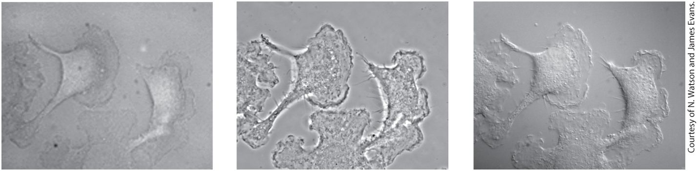
a medium-sized car — have a value approaching 1.5. Notice that the magnification is not part of this equation. Owing to limitations in the values of , , and based on the physical properties of light, the limit of resolution of a microscope using light of wavelength is about . No matter how many times the image is magnified, a conventional light microscope can never resolve objects that are closer than about apart or reveal details smaller than about in size. However, some newer and sophisticated technologies devised to overcome this resolution barrier can resolve objects that are just a few 10s of nanometers apart. We discuss such superresolution microscopes in a later section. Phase-Contrast and DifferentialInterference-Contrast Microscopy Visualize Unstained Live Cells Cells are about 70 percent water, 15 percent protein, and 6 percent RNA, and contain smaller amounts of lipids, DNA, and small molecules. Since none of these major classes of molecules are colored, and since they hardly impede the transmission of light, special methods must be used to see cells in a microscope. For example, the simplest microscopes view cells under bright-field optics (Figure 4-9b), and little detail can be seen (Figure 4-10, left). Two common methods for imaging live cells and unstained tissues to generate contrast take advantage of differences in the refractive index and thickness of cellular materials. These methods, called

phase-contrast microscopy and differential-interference-contrast (DIC) microscopy (or Nomarski interference microscopy), produce images that differ in appearance and reveal different features of cell architecture.

Figure 4-10 compares images of live, cultured cells obtained with these two methods and with standard bright-field microscopy. Since optical microscopes are expensive, they are often set up to perform many different types of microscopy on the same microscope stand (see Figure 49a–d).

FIGURE 4-10 Live cells can be visualized by microscopy techniques that generate contrast by interference. These micrographs show live, cultured macrophage cells viewed by bright-field microscopy (left), phase-contrast microscopy (middle), and differentialinterference-contrast (DIC) microscopy (right). In a phase-contrast image, cells are surrounded by alternating dark and light bands; in-focus and out-of-focus details are simultaneously imaged in a phase-contrast microscope. In a DIC image, cells appear in pseudorelief. Because only a narrow in-focus region is imaged, a DIC image is an optical slice through the object. Description The bright-field micrograph shows amorphous macrophage cells where the internal features are difficult to discern. The phase-contrast micrograph shows dark edges and bright internal features of the macrophage cells. The differential-interference contrast micrograph shows a three-dimensional view with slight peaks and valleys on the surface of each macrophage cell.

Phase-contrast microscopy generates an image in which the degree of darkness or brightness of a region of a specimen depends on the refractive index of that region. Light moves more slowly in a medium with a higher refractive index. Thus a beam of light is refracted (bent) once as it passes from the medium into a transparent object and again when it departs. In a phase-contrast microscope, a cone of light generated by an annular diaphragm in the condenser lens illuminates the specimen (see Figure 49c). The light passes through the specimen into the objective lens, and the unobstructed direct light passes through a region of the phase plate that both transmits only a small percentage of the light and changes its phase slightly. The part of a light wave that passes through a specimen will be refracted and will be out of phase (out of synchrony) with the part of the wave that does not pass through the specimen. How much their phases differ depends on the difference in refractive index along the two paths and on the thickness of the specimen. The refracted and unrefracted light is recombined at the image plane to form the image. If the two parts of the light wave are recombined, the resultant light will be brighter if they are in phase and less bright if they are out of phase (Figure 4-10, middle). Phasecontrast microscopy is suitable for observing single cells or thin cell layers, but not thick tissues. It is particularly useful for examining the location and movement of larger organelles in live cells. DIC microscopy, which is based on splitting the light into two perpendicular components before passing them through the specimen and then recombining them to observe their interference pattern, is the method of choice for visualizing extremely small details and thick objects. Contrast is generated by differences in the refractive index of the object

Imaging Subcellular Details Often Requires That Specimens Be Fixed, Sectioned, and Stained

and of its surrounding medium. In DIC images, objects appear to cast a shadow to one side. The shadow primarily represents a difference in the refractive index of a specimen rather than its topography. DIC microscopy easily defines the outlines of large organelles, such as the nucleus and vacuole. In addition to having a three-dimensional appearance, a DIC image is a thin optical section, or slice, through the object (Figure 4-10, right). Thus details of the nucleus in thick specimens (e.g., an intact Caenorhabditis elegans roundworm; see Figure 22-26d) can be observed in a series of such optical sections, and the three-dimensional structure of the object can be reconstructed by combining the individual DIC images. Both phase-contrast and DIC microscopy can be used in live cell microscopy, in which the same cell is imaged at regular intervals over time to generate a movie that allows the observer to study cell movement. Imaging Subcellular Details Often Requires That Specimens Be Fixed, Sectioned, and Stained As we have seen, live cells and tissues generally do not absorb light, so they are nearly invisible in a light microscope. Although cells can be visualized by the special techniques we have just discussed, these methods do not reveal the fine details of structure. Specimens for light microscopy are commonly fixed with a solution containing chemicals that cross-link most proteins and nucleic acids. Formaldehyde, a common fixative, cross-links amino groups on adjacent

molecules; these covalent bonds stabilize protein-protein and protein– nucleic acid interactions and render the molecules insoluble and stable for subsequent procedures. After fixation, a tissue sample for examination by light microscopy is usually embedded in paraffin and cut into sections about thick (Figure 4-11a). Cultured cells growing on glass coverslips are thin enough to be fixed in situ and visualized by light microscopy without the need for sectioning.

FIGURE 4-11 Tissues for light microscopy are commonly fixed, embedded in a solid medium, and cut into thin sections. (a) A fixed tissue is dehydrated by soaking in a series of alcohol-water solutions, ending with an organic solvent compatible with the embedding medium. To embed the tissue for sectioning, the tissue is placed in liquid paraffin. After the block containing the specimen has hardened, it is mounted on the arm of a microtome, and slices are cut with a knife. Typical sections cut for light microscopy are thick. The sections are collected on microscope slides and stained with an appropriate agent. (b) Sections of normal (top) and cancerous (adenocarcinoma, bottom) human colon stained with H&E stain. Notice the disorganization of the cells in the cancer tissue. Description The illustration shows a microtome with a specimen block attached to a specimen holder. Below the specimen holder is the knife used for thin slicing of the specimen. An enlarged view of the specimen holder shows the specimen block in a half-cut position and a cut section of the specimen. A microscope slide below the microtome contains four cut sections of the specimen. A micrograph labeled B on the top shows a section of the normal human colonic epithelium with goblet cells stained with H and E stain, and a micrograph at the bottom shows a section of cancerous dysplastic human colonic epithelial cells stained with H and E stain. Finally, a specimen for light microscopy is stained, allowing the main structural features of the cell or tissue to be clearly seen. Many chemical stains bind to molecules that have specific features. For example, histological samples are often stained with hematoxylin and eosin (“H&E stain”). Hematoxylin binds to basic amino acids (lysine and arginine) on many different kinds of proteins, whereas eosin binds to acidic molecules (e.g., DNA and side chains of the amino acids aspartate and glutamate). Because of their different binding properties, these dyes stain various cell types sufficiently differently that they are distinguishable visually (Figure 4-11b). If an enzyme catalyzes a reaction that produces a colored or

Intracellular Ion Concentrations Can Be Determined with Ion-Sensitive Fluorescent Dyes

otherwise visible precipitate from a colorless precursor, that enzyme can be detected in cell sections by their colored reaction products. Such staining techniques, although once quite common, have been largely replaced by other techniques for visualizing particular proteins, as we discuss next. Fluorescence Microscopy Can Localize and Quantify Specific Molecules in Live Cells Perhaps the most versatile and powerful technique for localizing molecules within a cell by light microscopy is fluorescent staining of cells and observation by fluorescence microscopy. A chemical is said to be fluorescent if it absorbs light at one wavelength (the excitation wavelength) and emits light (fluoresces) at a specific longer wavelength. Fluorescence microscopes allow the excitation light to pass through the objective lens into the sample and then permit the user to selectively observe the emitted fluorescent light coming back through the objective lens from the sample. This is achieved by using a special type of filter, called a dichroic mirror, that reflects the excitation light into the sample and allows the longer wavelength light emitted by the fluorescent sample to pass through to the observer (see Figure 4-9d). Here we discuss several ways in which fluorescence microscopy can be used to examine specific molecules in cells.

Intracellular Ion Concentrations Can Be Determined with Ion-Sensitive Fluorescent Dyes The concentration of or within live cells can be measured with the aid of fluorescent dyes, or fluorochromes, whose fluorescence depends on the concentration of these ions. As discussed in later chapters, intracellular and concentrations have pronounced effects on many cellular processes. For instance, many hormones and other stimuli cause a rise in cytosolic , from the resting level at less than M up to or M, that induces various cellular responses, such as the contraction of muscle. Introduction of the fluorochrome Fura-2, which binds a single , can be used to follow transient increases of in living cells. This binding, which is proportional to the cytosolic concentration over a certain range, increases the fluorescence of Fura-2 at one particular wavelength. At a second wavelength, the fluorescence of Fura-2 is the same whether or not is bound and thus provides a measure of the total amount of Fura-2 in a region of the cell. By examining cells continuously in the fluorescence microscope and measuring rapid changes in the ratio of Fura2 fluorescence at the two wavelengths, one can quantify rapid changes in the fraction of Fura-2 that has bound a ion, and thus in the concentration of cytosolic . Although Fura-2 has been used extensively to study levels, as we discuss later in this chapter, heterologous expression of a protein sensor, which becomes

fluorescent upon binding , has largely replaced the use of - sensitive dyes. Fluorescent dyes that are sensitive to concentrations can be used to monitor the cytosolic pH of live cells. Other useful probes consist of a fluorochrome linked to a weak base that is only partially protonated at neutral pH and thus can freely permeate cellular membranes. In acidic organelles, however, these probes become protonated. Because the protonated probes cannot recross the organelle membrane, they accumulate in the lumen at concentrations much greater than in the cytosol. Thus this type of fluorescent dye can be used to specifically stain particular organelles in live cells, such as lysosomes and mitochondria shown in Figure 4-12.

EXPERIMENTAL FIGURE 4-12 Location of lysosomes and mitochondria in a cultured living bovine pulmonary artery endothelial cell. The cell was stained with a greenfluorescing dye that is specifically bound to mitochondria and a red-fluorescing dye that is

Immunofluorescence Microscopy Can Detect Specific Proteins in Fixed Cells

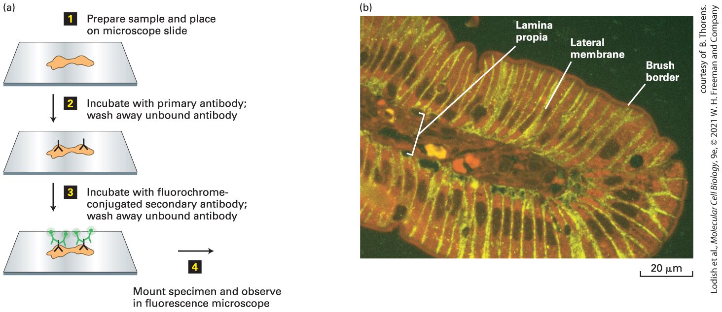
specifically incorporated into lysosomes. The image was sharpened using a deconvolution computer program discussed later in the chapter. N, nucleus. Description The fluorescence micrograph of a bovine pulmonary artery endothelial cell shows a large black circular region, nucleus surrounded by mitochondria and lysosomes. Mitochondria are stained green, and lysosomes are stained red. Immunofluorescence Microscopy Can Detect Specific Proteins in Fixed Cells The common chemical dyes mentioned above stain nucleic acids or broad classes of proteins, but it is much more informative to detect the presence and location of specific proteins. Immunofluorescence microscopy, the most widely used method of detecting specific proteins, uses an antibody to which a fluorescent dye has been covalently attached. To use this method, one must first generate antibodies to the specific protein of interest. As discussed briefly in Section 4.1 and in detail in Chapter 24, when an experimental animal is injected with an antigen, the vertebrate immune system responds by generating polyclonal antibodies that recognize different epitopes on the antigen. The antibodies that specifically recognize the antigen can be purified from all the other antibodies and proteins in blood serum by affinity chromatography over a resin on which the antigen is immobilized (see Figure 3-43c). Alternatively, as we described earlier in this chapter, it is possible to

generate a clonal cell line that secretes antibodies to a specific epitope on the antigen; these are called monoclonal antibodies. To use either type of antibody to localize a cytosolic protein, the cells or tissue must first be fixed to ensure that all components remain in place, and the cell must be permeabilized to allow entry of the antibody, which is commonly done by incubating the cells with a non-ionic detergent or by extracting the lipids with an organic solvent. To localize just a surface protein, the cell is fixed, but there is no need to permeabilize it. In one version of immunofluorescence microscopy, the antibody is covalently linked to a fluorochrome. Classically used fluorochromes include rhodamine and Texas red, which emit red light; Cy3, which emits orange light; and fluorescein, which emits green light; but newer and more photostable fluorochromes, with emission wavelengths from blue to farred, have now been developed. When a fluorochrome-antibody complex is added to a permeabilized cell or tissue section, the complex will bind to the corresponding antigen, then light up when illuminated at the excitation wavelength. Staining a specimen with different dyes that fluoresce at different wavelengths allows multiple proteins as well as DNA to be localized within the same cell. The most commonly used variation of this technique is called indirect immunofluorescence microscopy because the antibody specific to the protein of interest is detected indirectly. In this technique, an unlabeled monoclonal or polyclonal antibody is applied to the specimen, followed by a second, fluorochrome-tagged antibody that binds to the constant (Fc) segment of the first antibody. For example, a secondary antibody can be

generated by immunizing a goat with the Fc segment that is common to all rabbit immunoglobulin G antibodies. When coupled to a fluorochrome, this second antibody preparation (called goat–anti-rabbit) will detect any rabbit antibody used to stain a tissue or cell (Figure 4-13). Because several goat–anti-rabbit antibody molecules can bind to a single rabbit antibody molecule in a specimen, the fluorescence is generally much brighter than if a single fluorochrome-tagged antibody were used. This approach is often extended to do double-label fluorescence microscopy, in which two proteins can be visualized simultaneously. For example, two proteins can be visualized by indirect immunofluorescence microscopy using primary antibodies made in different animals (e.g., rabbit and chicken) and secondary antibodies (e.g., goat–anti-rabbit and sheep–anti-chicken) labeled with different fluorochromes. In another variation, one protein can be visualized by indirect immunofluorescence microscopy and the second protein by a dye that specifically binds to it. Once the individual images are taken on the fluorescence microscope, they can be merged electronically (Figure 4-14, and see chapter-opening figure).

FIGURE 4-13 A specific protein can be localized in fixed tissue sections by indirect immunofluorescence microscopy. (a) To localize a protein by immunofluorescence microscopy, a tissue section, or sample of cells, must be chemically fixed and made permeable to antibodies (step 1 ). The sample is then incubated with a primary antibody that binds specifically to the antigen of interest, and unbound antibody is then removed by washing (step 2 ). The sample is next incubated with a fluorochrome-labeled secondary antibody that specifically binds to the primary antibody, and again, excess secondary antibody is removed by washing (step 3 ). The sample is then mounted in specialized mounting medium and examined in a fluorescence microscope (step 4 ). (b) In this example, a section of the rat intestinal wall was stained with Evans blue, which generates a nonspecific red fluorescence, and GLUT2, a glucose transport protein, was localized by indirect immunofluorescence microscopy. GLUT2 (yellow) is seen to be present in the basal and lateral sides of the intestinal cells, but is absent from the brush border, composed of closely packed microvilli on the apical surface facing the intestinal lumen. Capillaries run through the lamina propria, a loose connective tissue beneath the epithelial layer. [Part (b) from B. Thorens et al., 1990, Am. J. Physiol. 259:C279;] Description The illustration labeled A shows the four stages in fluorescent labeling. Stage 1: Prepare sample and place on a microscope slide. Stage 2: Incubate with primary antibody; wash away unbound antibody. Stage 3: Incubate with fluorochrome-conjugated secondary antibody; wash away unbound antibody. Stage 4: Mount specimen and observe in a fluorescence microscope. The micrograph labeled B shows a section of finger-shaped rat intestinal cells. The central region is labeled lamina propia. To the right is a thick outer region labeled lateral membrane. To the right of the lateral membrane is a thin outermost border labeled brush border. The yellow fluorescence between the basal and lateral sides of the intestinal cells represents glucose transport protein.

EXPERIMENTAL FIGURE 4-14 Double-label fluorescence microscopy can visualize the relative distributions of two proteins. In double-label fluorescence microscopy, each protein must be labeled with a different fluorochrome. (a) A cultured cell was fixed and permeabilized and then incubated with Rhodamine-labeled phalloidin, a reagent that specifically binds to filamentous actin. It was also incubated with rabbit antibodies to tubulin, the major component of microtubules, followed by a fluorescein-labeled secondary goat–anti-rabbit antibody. (b) The upper panels show the fluorescein-stained tubulin (left) and Rhodamine-stained actin (right), and the lower panel shows the electronically merged images. Description The illustration labeled A shows microtubules, a hollow cylinder of tubulin proteins labeled with primary antibodies (rabbit, black) that recognize microtubules and fluorochrome-conjugated secondary antibodies (goat–anti-rabbit, green). Above the microtubule is the actin filaments, helical polymers of actin protein tagged with Rhodamine-labeled phalloidin (fluorochrome-conjugated drug that binds actin filaments, red). The micrograph labeled B shows fluorescein stained tubulin (green) on the top left and Rhodamine stained actin (red) on the top right. At the bottom is an electronically merged fluorescein stained tubulin and Rhodamine stained actin. In another widely used version of this technology, molecular genetic techniques are used to make a cDNA encoding a recombinant protein to which is fused a short sequence of amino acids called an epitope tag. When expressed in cells, this cDNA will generate the protein linked to the specific tag. Two commonly used epitope tags are FLAG, which encodes the amino acid sequence DYKDDDDK (single-letter amino acid code), and Myc, which encodes the sequence EQKLISEEDL. Commercial fluorochrome-coupled monoclonal antibodies to the FLAG or Myc epitopes can then be used to detect the recombinant protein in the cell. In an extension of this technology to allow the simultaneous visualization of

Tagging with Fluorescent Proteins Allows the Visualization of Specific Proteins in Live Cells

two proteins, one protein can be tagged with FLAG and a different protein with Myc. Each tagged protein is then visualized with a different color, for example, with a labeled antibody emitting green light for the Myc epitope and a labeled antibody emitting red light to the FLAG epitope. One has to use caution in studying expressed tagged proteins to ensure that the tag does not interfere with the protein’s function or location. Tagging with Fluorescent Proteins Allows the Visualization of Specific Proteins in Live Cells The jellyfish Aequorea victoria expresses a naturally fluorescent protein, called green fluorescent protein (GFP, ~27 kDa). GFP contains a serine, tyrosine, and glycine sequence whose side chains spontaneously cyclize to form a green-fluorescing fluorochrome when illuminated with blue light. Using recombinant DNA technology, it is possible to make a DNA construct in which the coding sequence of GFP is fused to the coding sequence of a protein of interest. When this construct is introduced into and expressed in cells, a GFP-tagged protein is made in which the protein of interest is covalently linked to GFP as part of the same polypeptide. Although GFP is a medium-sized protein, the function of the protein of interest is often not changed by fusing it to GFP. This technique allows one to visualize GFP — and hence the location of the protein of interest. Not only can we see the location of the GFP-tagged protein immediately but we can also view its distribution in a live cell over time and thereby assess its dynamics or track its localization following various treatments, such as

the application of specific drugs. The simple idea of tagging specific proteins with GFP revolutionized cell biology and led to the subsequent development of many different fluorescent proteins (Figure 4-15). Use of this colorful variety of fluorescent proteins allows one to visualize two or more proteins simultaneously if they are each tagged with a differentcolored fluorescent protein. We describe additional techniques that exploit fluorescent proteins in the following sections.

FIGURE 4-15 Many different colors of fluorescent proteins are available. (a) Tubes show the emission colors and names of many different fluorescent proteins. (b) An agar dish is illuminated to show growing bacteria expressing several different-colored fluorescent proteins. Description The illustration labeled A shows fifteen Eppendorf tubes arranged from left to right containing different fluorescent proteins in different colors. The fluorescent proteins

Deconvolution and Confocal Microscopy Enhance Visualization of Three-Dimensional Fluorescent Objects

and their colors are as follows: m plum, plum; m Grape 2, red wine; m-Raspberry, violet; m-Grape 1, red; m Cherry, cherry violet; m Strawberry, strawberry red; m Tangerine, orange; t d Tomato, pale orange; m orange, yellow-orange; m banana, yellow; m honeydew, green-yellow; citrine, lime green; E G F P, green; E C F P, sky blue; E B F P, blue. The illustration labeled B shows a beach view streaked in a petri dish using several bacteria producing different colored fluorescent proteins. Deconvolution and Confocal Microscopy Enhance Visualization of Three-Dimensional Fluorescent Objects Conventional fluorescence microscopy has two major limitations. First, the fluorescent light emitted by a sample comes not only from the plane of focus but also from molecules above and below it; thus the observer sees a blurred image caused by the superposition of fluorescent images from molecules at many depths in the cell. The blurring effect makes it difficult to determine the actual spatial arrangements. Second, to visualize thick specimens, consecutive (serial) images at various depths throughout the sample must be collected and then aligned to reconstruct structures in the original thick tissue. Two general approaches have been developed to obtain high-resolution three-dimensional information. Both of these methods require that the image be collected electronically so that it can then be computationally manipulated as necessary.

The first approach, called deconvolution microscopy, uses computational methods to remove fluorescence contributed by out-of-focus parts of the sample. Consider a three-dimensional sample in which images from three different focal planes are recorded. Since the whole sample is illuminated, the image from plane 2 will contain out-of-focus fluorescence from planes 1 and 3. If we knew exactly how out-of-focus fluorescence from planes 1 and 3 contributed to the light collected in plane 2, we could computationally remove it. To obtain this information for a particular microscope, we can make a series of images of focal planes from a test slide containing tiny fluorescent beads. Each bead represents a pinpoint of light that becomes a blurred object outside its focal plane; from these images we can determine a point spread function that enables us to calculate the distribution of fluorescent point sources that contributed to the blur when out of focus. Once we have calibrated the microscope in this manner, the experimental series of images can be computationally deconvolved. Microscopes with automated stages to collect the images, and associated software programs to deconvolve the images, are available commercially. Images restored by deconvolution display impressive detail without any blurring, as illustrated in Figure 4-16.

EXPERIMENTAL FIGURE 4-16 Deconvolution fluorescence microscopy yields highresolution optical sections. A cultured cell in mitosis was stained with fluorochromelabeled reagents specific for DNA (blue), microtubules (green), and the microfilamentmembrane linking protein ezrin (red). A series of fluorescent images were obtained at consecutive focal planes (optical sections) through the cell. A single plane is shown in which the left half is a raw image and the right half has been subjected to deconvolution processing. Notice how much clearer the chromosomes (blue) and microtubules (green) are after processing. Description

The left half of the figure is the raw image and is blurry. The right half has undergone deconvolution processing and the stained structures are sharp. In the center, the chromosomes are blue and the microtubules are green. Around the perimeter of the cell, the protein ezrin is stained red. The second approach to obtaining better three-dimensional information is called confocal microscopy because it uses optical methods to obtain images from a specific focal plane and exclude light from other planes. Confocal microscopes collect a series of images focused through the vertical depth of the sample, from which an accurate three-dimensional representation can be computationally generated. Two types of confocal microscopes are in common use today, a point-scanning confocal microscope (also known as a laser-scanning confocal microscope, or LSCM) and a spinning disk confocal microscope. The idea behind each microscope is to both illuminate and collect emitted fluorescent light from just one small area of a focal plane at a time in such a way that out-offocus light is excluded. This can be achieved by collecting the emitted light through a pinhole before it reaches the detector — light from the illuminated focal plane passes through, whereas light from other focal planes is largely excluded. The illuminated area is then moved across the whole focal plane to build up the image electronically. The two types of microscopes differ in how they cover the image. The point-scanning microscope uses a point laser light source at the excitation wavelength to rapidly scan the focal plane in a raster pattern, collects the emitted fluorescence in a photomultiplier tube, and thereby builds up an image (Figure 4-17a). It can then take a series of images at different depths in the sample to generate a three-dimensional reconstruction. A point-scanning

confocal microscope can provide exceptionally high-resolution images in both two and three dimensions (Figure 4-18), although it has two minor limitations. First, it can take significant time to scan each focal plane, so if a very dynamic live cell process is being imaged, the microscope may not be able to collect images fast enough to follow the dynamics. Second, it illuminates each spot with intense laser light, which can bleach the fluorochrome being imaged and damage live cells by phototoxicity, thereby limiting the number of images that can be collected.

FIGURE 4-17 Light paths for two types of confocal microscopy. Both types of microscopy are assembled around a conventional fluorescence microscope (yellow shading). (a) Light path in a point-scanning confocal microscope. A single-wavelength point of light from an appropriate laser is reflected off a dichroic mirror and bounces off two scanning mirrors and from there passes through the objective lens to illuminate a spot in the specimen. The scanning mirrors rock back and forth in such a way that the light scans the specimen in a raster fashion (see green lines in the specimen). The fluorescence emitted by the specimen passes back through the objective lens and is bounced off the scanning mirrors and through the dichroic mirror. This allows the light to pass toward the pinhole. This pinhole excludes light from out-of-focus focal planes, so the light reaching the

photomultiplier tube comes almost exclusively from the illuminated spot in the focal plane. A computer then takes these signals and reconstructs the image. (b) Light path in a spinning disk confocal microscope. Here, instead of using two scanning mirrors, the beam from the laser is spread to illuminate pinholes on the coupled spinning disks, the first consisting of microlenses to focus the light on pinholes in the second disk. The excitation light passes through the objective lens to provide point illumination of a number of spots in the specimen. The fluorescence emitted passes back through the objective lens and through the holes in the spinning disk, and is then bounced off a dichroic mirror into a sensitive digital camera. The pinholes in the disk are arranged so that as it spins, it rapidly illuminates all parts of the specimen several times. As the disk spins as fast as 5000 rpm, very dynamic events in live cells can be recorded. Description Both types of the microscope are assembled around a conventional fluorescence microscope. The illustration labeled A shows a single-wavelength point of light from a laser entering the scanning head unit of the point scanning confocal microscope. The scanning head unit comprises dichroic mirror, scanning mirror in y dimension, scanning mirror in x dimension, pinhole, and a photomultiplier tube. The light from the laser is reflected off a dichroic mirror, bounces off scanning mirror in y dimension and scanning mirror in x dimension, and passes through the objective lens to illuminate a spot in the specimen. The scanning mirrors rock back and forth such that the light scans the specimen in a raster fashion (green lines in the specimen). The fluorescence of the specimen passes back through the objective lens and bounces off the scanning mirrors and through the dichroic mirror, allowing the light to pass toward the pinhole. The pinhole excludes light from out-of-focus focal planes, so the light reaching the photomultiplier tube comes almost exclusively from the illuminated spot in the focal plane. A computer then takes these signals and reconstructs the image. The illustration labeled B shows a beam of lights from a laser entering the spinning disk head unit of the spinning disk head confocal microscope. The spinning disk head unit comprises a microlens array, dichroic mirror, and pinhole array. The beam of lights from the laser is spread to illuminate pinholes on the coupled spinning disks, the first consisting of microlenses that focus the light on pinholes in the second disk. The excitation light passes through the objective lens to provide point illumination of several spots in the specimen. The fluorescence passes back through the objective lens, through the holes

in the spinning disk, and is bounced off a dichroic mirror into a sensitive digital camera connected to a computer.

FIGURE 4-18 Confocal microscopy produces an in-focus optical section through thick cells. A mitotic fertilized egg from a sea urchin (Psammechinus) was lysed with a detergent, exposed to a tubulin antibody, and then exposed to a fluorescein-tagged antibody that binds to the anti-tubulin antibody. (a) When viewed by conventional fluorescence microscopy, the mitotic spindle is blurred. This blurring occurs because background fluorescence is detected from tubulin above and below the focal plane as depicted in the sketch. (b) The confocal microscopic image is sharp, particularly in the center of the mitotic spindle. In this case, fluorescence is detected only from molecules in the focal plane, generating a very thin optical section. [Micrographs © 1987 White et al., J. Cell Biol. 105:41–48. https://doi.org/10.1083/jcb.105.1.41] Description A conventional fluorescence micrograph labeled A shows a blurred mitotic spindle, and an illustration below the micrograph shows tubulin above and below the focal plane. The imaged volume is larger than the focal plane. A confocal fluorescence micrograph labeled B shows a sharp mitotic spindle, and an illustration below the

micrograph shows tubulin on the focal plane. The imaged volume and the focal plane remains the same. The spinning disk microscope circumvents these two limitations (Figure 4-17b). The excitation light from a laser is spread out and illuminates a small part of a disk spinning at high speed; for example, at 5000 rpm. The disk in fact consists of two linked disks: one with 20,000 lenses that precisely focuses the laser light on 20,000 pinholes of the second disk. The pinholes are arranged in such a way that they completely scan the focal plane of the sample several times with each turn of the disk. The emitted fluorescent light returns through the pinholes of the second disk and is reflected by a dichroic mirror and focused onto a highly sensitive digital camera. In this way, the sample is scanned in less than a millisecond, so the real-time location of a fluorescent reporter can be captured even if it is highly dynamic (Figure 4-19). A limitation of the spinning disk microscope is that the pinhole size is generally fixed and has to be matched to the magnification of the objective lens, so it is generally configured for use with a or objective and is less useful for the lower magnification imaging that might be required in tissue sections. However, recently, spinning disk head units have become available in which the pinhole size can be changed to better accommodate objectives with other magnifications. Thus the point-scanning and spinning disk confocal microscopes have overlapping and complementary strengths.

Two-Photon Excitation Microscopy Allows Imaging Deep into Tissue Samples

EXPERIMENTAL FIGURE 4-19 The dynamics of microtubules can be imaged on the spinning disk confocal microscope. Six frames from a movie of GFP-tubulin in two rodshaped cells of fission yeast are shown. Arrowheads indicate examples of shrinking and growing microtubules. Description The six frames of the spinning disk confocal micrograph show the movement of microtubules in two rod-shaped cells of yeast under various time series. The movements of the microtubules are captured at 0, 30, 58, 85, 113, and 140 seconds. White and orange arrowheads point out the shrinking and growing microtubules. Two-Photon Excitation Microscopy Allows Imaging Deep into Tissue Samples We have just seen how point-scanning confocal microscopy can help reduce fluorescence from out-of-focus planes. To achieve this, it focuses a cone of laser light on a spot that scans across the focal plane. Regions above and below the focal plane are also illuminated by this cone of light, generating an out-of-focus signal that must be removed by collecting the light through a pinhole. This intense cone of light can also lead to photobleaching (rendering the fluorescent protein inactive) or damage to the sample by phototoxicity. If the sample is very thin, these are not significant problems, but as the sample gets thicker, they become more relevant. To circumvent these problems, use was made of the finding that a fluorochrome can be excited either by a single photon — for example, at

488 nm — or by two photons of half the energy at 960 nm, either of which will generate the same emission wavelength (Figure 4-20a). Thus if a 960 nm cone of laser light is focused on a spot in one plane so that only at the focal point is there sufficient density of photons to excite the fluorochrome (Figure 4-20b), no out-of-focus signal will be obtained and less photobleaching or phototoxicity will occur. Because only fluorochromes in the focal plane are excited, two-photon microscopy can be used to explore much thicker samples, and there is no need for a pinhole to exclude out-of-focus light. Moreover, 960-nm light can penetrate more deeply into biological material than can 488-nm light. However, very high laser intensity is required for two-photon excitation microscopy, as the two photons must arrive within about a femtosecond of each other, which is achieved using rapid laser pulses. If individual cells in an animal express different color variants of fluorescent proteins, twophoton microscopy can be used to observe events in living animals (called intravital imaging) within about 1 mm of the surface (Figure 4-20c).

FIGURE 4-20 Two-photon excitation microscopy restricts illumination to the focal plane to allow deep penetration for intravital imaging. (a) Different excitation methods are used for conventional point-scanning confocal microscopy and for two-photon excitation microscopy. In the conventional system, absorption of a single photon of the appropriate wavelength (here at 488 nm, blue arrow) causes an electron to jump to the excited state. After undergoing vibrational relaxation (black dashed arrow), the electron falls back to the ground state with emission of one photon at a longer (lower energy) wavelength, in this case 507 nm (green arrow). In two-photon excitation, when two photons of the appropriate wavelength (shown here at 960 nm, red arrows) arrive almost instantaneously, they can both be absorbed and induce the electron to jump to the excited state. The electron undergoes some vibrational relaxation (black dashed arrow) and falls back to the ground state with the emission of a photon (507 nm). (b) A cuvette of fluorescent material is illuminated with 488-nm light (left), as in conventional confocal microscopy, or with intense 960-nm light, as in two-photon microscopy. Notice that the conventional system produces a bright cone of excitation outside the focal plane, whereas two-photon excitation illuminates just one spot in the focal plane. (c) An example of intravital imaging in which labeled neurons in a lobster were imaged.

TIRF Microscopy Provides Exceptional Imaging in One Focal Plane

[Part (b) Reprinted by permission from Nature Publishing Group, from Zipfel, W. R., et al. 2003. “Nonlinear magic: multiphoton microscopy in the biosciences,” Nat. Biotechnol., 21:1369–1377; permission conveyed through Copyright Clearance Center, Inc.; part (c) unpublished data from Peter Kloppenburg and Warren R. Zipfel.] Description The illustration on the left, labeled A shows excitation methods in point-scanning confocal microscopy with three horizontal lines and a black dot at the bottom line representing the electrons at the ground state. Excitation photon (blue arrow with 488 nanometers wavelength) activates the electron. The vertical line arises from the electron and reaches the top horizontal line of the six horizontal lines representing the electron at the excited state. The electron undergoes vibrational relaxation and falls back to the ground state with the release of emission photon (green arrow, 507 nanometers wavelength). The illustration on the right shows excitation methods in two-photon excitation microscopy with three horizontal lines and a black dot at the bottom line representing the electrons at the ground state. Excitation photons 1 and 2 (red arrow with 960 nanometers wavelength) activates the electron. The vertical line arises from the electron and reaches the top horizontal line of the six horizontal lines representing the electron at the excited state. The electron undergoes vibrational relaxation and falls back to the ground state with the release of emission photon (green arrow, 507 nanometers wavelength). The illustration labeled B on the left shows a cuvette filled with fluorescent materials and illuminated with 488 nanometers light. The bright cone of excitation scatters outside the focal cone. The illustration labeled B on the right shows a cuvette filled with fluorescent materials and illuminated with two 960 nanometers light. A single spot illuminates in the focal cone. The emission photons at the focal plane are 507 nanometers wavelength for both microscopy techniques. Intravital imaging labeled C shows the different colors of fluorescent proteins in the neurons of a lobster. TIRF Microscopy Provides Exceptional Imaging in One Focal

Plane The confocal microscopes we have just described provide amazing and informative images, but they are not perfect. Scientists continue to develop systems that are optimized for special circumstances. Some experimental situations call for fluorescence imaging in a thin focal plane adjacent to a surface, where it would be optimal to minimize out-of-focus background. For example, confocal imaging is not ideal for exploring the details of proteins at adhesion sites between a cell and a coverslip, or for following the kinetics of assembly of microtubules attached to a coverslip. Both of these situations can be imaged at high sensitivity using total internal reflection fluorescence (TIRF) microscopy, in which only the portion of the specimen immediately adjacent to the coverslip is illuminated. In the most common configuration of TIRF microscopy, the excitation light comes through the objective lens. However, the angle at which the light arrives at the coverslip is adjusted to be slightly larger than the critical angle so that the light is reflected off the coverslip and returns up through the objective (Figure 4-21a). This generates a narrow band of light, called an evanescent wave, that illuminates only about 50– 100 nm of the sample adjacent to the coverslip (2–4 times the thickness of a microtubule), with no illumination of the rest of the sample. Thus if you have a complex mixture of fluorescent structures in a specimen, the TIRF microscope will show you only those that are within 50–100 nm of the coverslip. TIRF has been exceptionally useful in identifying structures on the bottoms of cells grown on a coverslip (Figure 4-21b) and for

measuring the kinetics of assembly and disassembly of structures such as microtubules and actin filaments (see Chapters 17 and 18). EXPERIMENTAL FIGURE 4-21 Fluorescent samples in a restricted focal plane can be imaged by total internal reflection fluorescence (TIRF) microscopy. (a) Illumination setup for TIRF microscopy. The angle at which light becomes reflected from a glass-water interface is called the critical angle . Below this angle, the beam of light will pass into the specimen; above , it will be reflected. In TIRF microscopy, the angle of the incident beam , resulting in most of the light being reflected, but also generating a very thin region of illumination called the evanescent wave (depicted in light green). (b) Immunofluorescence microscopy with tubulin antibody was used to visualize microtubules viewed by

FRAP Reveals the Dynamics of Cellular Components

conventional fluorescence microscopy (top) and by TIRF (middle), and a merged image was created from the two views (bottom). The two images were collected and false-colored red and green so that the merge could highlight those microtubules that are close to the coverslip (green). [Part (b) © 2010 J. B. Manneville et al., 2010, J. Cell Biol. 191:585–598. https://doi.org/10.1083/jcb.201002151] Description The illustration labeled A shows a coverslip with a specimen and an incident light falls on the coverslip and reflects. The perpendicular line from the specimen shows the angle theta, which is larger than the critical angle theta c. The evanescent wave is formed over the specimen and illuminates only about 50 to 100 nanometers of the specimen adjacent to the coverslip. The illustration labeled B shows three micrographs. The first conventional fluorescence micrograph shows microtubules. The second total internal reflection fluorescence micrograph shows microtubules. The third micrograph shows a merged image of the first two micrographs and false-colored with red and green. The green highlights the microtubules near the bottom of the coverslip. A scale bar reads 5 micrometers. FRAP Reveals the Dynamics of Cellular Components Live cell fluorescence imaging reveals the locations and bulk dynamics of populations of fluorescent molecules, but it doesn’t tell you how dynamic individual molecules are. For example, if we see that a GFP-labeled protein forms a patch at the surface of a cell, does this represent a stable collection of fluorescent protein molecules or a dynamic equilibrium, with fluorescent proteins coming in and out of the patch? We can investigate

this question by observing the dynamics of the molecules in the patch (Figure 4-22). If we use a high-intensity light to permanently bleach the fluorochrome (e.g., GFP) in the patch, initially there will be no fluorescence coming from it, and it will look dark in the fluorescence microscope. However, if the components in the patch are in dynamic equilibrium with unbleached molecules elsewhere in the cell, the bleached molecules will be replaced by unbleached ones, and the fluorescence will begin to come back. The rate of fluorescence recovery is a measure of the dynamics of the molecules. This technique, known as fluorescence recovery after photobleaching (FRAP), has revealed how very dynamic many components of cells are. For example, it has been used to determine the diffusion coefficient of cytoskeletal and membrane proteins (see

Figure 10-10). In another approach to measuring the dynamics of tagged proteins, variants of fluorescent proteins have been developed that can be switched, using a laser of an appropriate wavelength, from emitting green light to emitting red light. In this way, the dynamics of the switched population of red-emitting molecules can be imaged in live cells.

EXPERIMENTAL FIGURE 4-22 Fluorescence recovery after photobleaching (FRAP) reveals the dynamics of molecules. In a live cell, following the distribution of a GFPlabeled protein provides a view of the overall distribution of the protein, but it doesn’t tell us how dynamic populations of individual molecules might be. (a) In FRAP, the GFP fluorochrome is bleached by a short burst of strong laser light focused on the region of interest (ROI). The light rapidly bleaches the molecules irreversibly, so they are not detected again. Restoration of fluorescence in the region tells us that unbleached molecules have moved into the ROI. (b) FRAP was used to determine the exchange rate of EBP50 and ezrin, two components of microvilli (seen as white lines), on the apical surface of epithelial cells. In cells expressing either GFP-EBP50 or ezrin-GFP, the GFP in a small region indicated by the green box was bleached, and recovery by exchange with unbleached protein was followed. The fluorescence of GFP-EBP50 returns very fast, indicating it has a fast exchange rate, whereas the fluorescence of ezrin-GFP returns slowly, indicating a slower exchange rate. (c) By quantifying the recovery, the dynamic properties of EBP50 and ezrin can be established.

FRET Measures Distance Between Fluorochromes

[Parts (b) and (c) ©2012 D. Garbett and A. Bretscher, 2012, J. Cell Biol. 198:195–203. https://doi.org/10.1083/jcb.201204008] Description The illustration labeled A shows the time taken for the recovery of fluorescence after photobleaching. At the top is a Green fluorescent protein, fluorochrome, followed by the same fluorochrome bleached with strong laser light at the region of interest (R O I). A black dot is seen on the R O I after the exposure to light. The molecules show a gradual decrease in the intensity of the black dot over time. The recovery of fluorescence over time in seconds at the R O I are as follows: 5, Dark black spot; 10, black spot; 15, light black spot; 30, gray spot. The illustration labeled B shows Ezrin- G F P and G F P- E B P 50 components of microvilli on the apical surface of epithelial cells. A green box indicates the portion of the bleached cell. The recovery of fluorescence over time in seconds at the bleached area of Ezrin- G F P are as follows: 5, No recovery; 10, No recovery; 15, very little recovery; 30, little recovery. The recovery of fluorescence over time in seconds at the bleached area of G F P- E B P 50 are as follows: 5, very little recovery; 10, little recovery; 15, little recovery; 30, half recovery. The graph labeled C shows the intensities of G F P E-B P 50 and Ezrin G F P. The vertical axis plots normalized intensity and ranges from 0 to 1 in increments of 0.2. The horizontal axis plots time post bleach and ranges from 0 to 40 in increments of 40. The data are approximate. Ezrin- G F P starts at (0, 0.25), increases gradually, and ends at (45, 0.6). G F P-E B P 50 starts at (0, 0.25) increase gradually and ends at (45, 0.90). FRET Measures Distance Between Fluorochromes Fluorescence microscopy can also be used to determine if two proteins interact in vivo by taking advantage of a phenomenon called Förster resonance energy transfer (FRET). This technique uses a pair of fluorescent proteins in which the emission wavelength of the first is close

to the excitation wavelength of the second (Figure 4-23a). For example, when cyan fluorescent protein (CFP) is excited with 433-nm light, it fluoresces and emits light at 475 nm. If yellow fluorescent protein (YFP) is close by, however, instead of emitting 475-nm light, CFP transfers energy to YFP by FRET, and YFP emits light at 530 nm. The efficiency of FRET is proportional to , where is the distance between the fluorochromes; it is therefore very sensitive to small changes in distance and in practice is not detectable at distances greater than 10 nm. Thus by illuminating an appropriately prepared sample with 433-nm light and observing at 530 nm, one can tell if proteins separately tagged with CFP and YFP are in very close proximity. For example, FRET sensors have been developed to determine where signaling between a small GTPbinding regulatory protein and its effector occurs in the cell (Figure 423b).

FIGURE 4-23 Protein-protein interactions can be visualized by FRET. The idea behind FRET is to use two different fluorescent proteins so that when one is excited, energy will be transferred to the second one by FRET, provided that they are sufficiently close. (a) In this example, cyan fluorescent protein (CFP) is fused to protein X, yellow fluorescent protein (YFP) is fused to protein Y, and both proteins are expressed in a live cell. If the cell is now illuminated with 433-nm light, the CFP will emit a fluorescent signal at 475 nm. If YFP is not close by (left), energy transfer will not occur, and no 530-nm light will be emitted. However, if protein X interacts with protein Y (right), it will bring CFP close to YFP, energy will be transferred to YFP by FRET, and YFP will emit light at 530 nm. (b) In this mouse fibroblast, FRET has been used to reveal that the interaction between an active regulatory protein (Rac) and its binding partner is localized to the front of the migrating cell. [Part (b) ©2003 R. B. Sekar and A. Periasamy, 2003, J. Cell Biol. 160:629–633. https://doi.org/10.1083/jcb.200210140]

Description The illustration labeled A shows a cyan fluorescent protein (C F P) fused with protein X absorbs light at 433 nanometers and emits light at 475 nanometers and a yellow fluorescent protein (Y F P) fused with protein Y. The interaction between X and Y proteins are not observed. Once when there is an interaction between the X and Y proteins, C F P, Y F P attaches, and the energy transfer occurs from C F P to Y F P by F R E T. During energy transfer, Y F P emits light at 530 nanometers. A F R E T image labeled B shows the active regulatory proteins (R a c) of mouse fibroblast. A color scale shows the ranges from low calcium ions to high calcium ions and a scale bar reads 10 micrometers. A clever application of FRET, called a FRET biosensor, can be used to sense local biochemical environments in live cells. The idea is to express a single polypeptide containing both CFP and YFP separated by a region that undergoes a conformational change when it senses a biochemical signal. In the absence of the signal, CFP and YFP are too far apart to undergo significant FRET. However, when the signal is detected, the conformational change brings CFP and YFP close enough together to generate FRET. A version of this technique can be used to measure the local activity of a specific protein kinase. In this case, between the CFP and YFP lies a region of polypeptide containing the substrate for the protein kinase — the sensor domain — and a domain that binds specifically to the phosphorylated substrate — the ligand domain (Figure 4-24a). When the sensor domain is phosphorylated by the kinase, the ligand domain binds to it and brings the CFP and YFP sufficiently close to undergo FRET. Since protein phosphorylation is a dynamic process, dephosphorylation of the sensor domain by the appropriate phosphatase will deactivate the FRET biosensor. Thus the FRET signal will reflect the

regions of the cell where there is excess kinase over phosphatase activity. As an example, scientists have developed a FRET biosensor for protein kinase A activity, which is activated by elevation of the signaling molecule cAMP (see Section 15.1). In cells expressing the protein kinase A biosensor, pharmacological elevation of cAMP induces rapid FRET (Figure 4-24b). Creative researchers are developing FRET biosensors to illuminate many different types of local environments; for example, FRET biosensors exist to measure the concentration and location of (see

Figure 4-27) and the activation state of GTPase switch proteins (see Figure 3-35).

Optogenetics Allows Light to Regulate Events in a Spatial and Temporal Manner

EXPERIMENTAL FIGURE 4-24 FRET biosensors can detect local biochemical environments. (a) A FRET biosensor is a fusion protein containing two fluorescent proteins linked by a region sensitive to the environment under study. In this example, a protein construct consists of CFP linked to YFP by a region that contains a particular sequence that can be phosphorylated by a specific kinase (the sensor domain) and a region (the ligand domain) that binds the sensor domain when it is phosphorylated. In the absence of kinase activity, the two fluorescent proteins are too far apart to undergo FRET, whereas when locally phosphorylated by the active kinase, the sensor domain becomes phosphorylated, the ligand domain binds to it, and CFP and YFP are brought sufficiently close to undergo FRET. The sensor can also be deactivated when it encounters the appropriate phosphatase that removes the added phosphate. Thus the biosensor reports on the ratio of kinase to phosphatase activity in the local environment. (b) An example of the use of a FRET biosensor for protein kinase A, which is activated by elevation of cAMP. In this example, forskolin, a drug that induces the generation of cAMP, was added to cells at and the images collected at various times thereafter. Imaging shows both the rate of activation and localization of the active kinase. [Part (b) from J. Zhang et al., 2001, Proc. Nat’l. Acad. Sci. USA 98:14997–15005. © 2001 National Academy of Sciences, U.S.A.] Description The illustration labeled A shows two proteins. One, the ligand domain, binding a phosphorylated substrate and the other, the sensor domain, acting as the substrate for kinase. The ligand domain is bound to C F P, which absorbs at 433 nanometers and emits at 475 nanometers. On the action of a protein kinase, the two domains interact, bringing the fluorescent proteins together and allowing FRET to occur, resulting in emission at 530 nanometers. The F R E T image labeled B shows the increase in F R E T color with time. The time in minutes and the colors are as follows: 0 minutes, Blue; 1.1 minutes, cyan; 1.4 minutes, green; 1.7 minutes, yellow; 2 minutes, orange; 3 minutes, red.

Optogenetics Allows Light to Regulate Events in a Spatial and Temporal Manner The idea that light can be used to control biochemical reactions in living cells arose from the study of phototaxis (attraction to light) of the green alga Chlamydomonas reinhardtii. Scientists discovered that a pulse of bright light induced the opening of a cation channel in a protein now known as channelrhodopsin. When channelrhodopsin is expressed in neurons, the opening of the channel by light allows the very rapid influx of that depolarizes the membrane. As we will see in Chapter 23, expression of channelrhodopsins in specific neurons combined with localized pulses of light can be used to dissect neural circuits. In a subsequent advance, methods were developed to use light to control biochemical reactions locally. This technology grew out of the identification of proteins that control plant phototropism (orientation toward, or away, from light). One of these, using the light sensitive LOV domain, has been extensively used. In an example to demonstrate the utility of this approach, light was used to induce an engineered protein located in the nucleus to move into the cytoplasm. As described in Chapter 13, proteins that are targeted to the nucleus contain a short nuclear localization sequence (NLS), and those that are exported from the nucleus have a short nuclear export sequence (NES) that can interact with a protein called an exportin to transport it out into the cytoplasm. A multidomain construct was made containing the following parts: Fluorescent protein-

NLS-LOV-NES (Figure 4-25a). The construct was made so that in the dark the NLS sequence was accessible, whereas the NES was masked. When expressed in cells in the dark, the protein is located in the nucleus as expected because NES cannot interact with exportin (Figure 4-25a, top). However, when illuminated, the LOV domain changes conformation, releasing the NES, which can now bind exportin (Figure 4-25a, bottom). This change results in export of the protein from the nucleus. When the illumination is turned off, the LOV domain reverses its conformation, masking the NES, and the protein returns to the nucleus (Figure 4-26b). If instead of the fluorescent protein a nuclear regulator was made part of the construct, this would allow light-mediated regulation of its activity. This type of approach has been used in many different settings, for example, to recruit proteins to the plasma membrane or to activate signaling pathways. EXPERIMENTAL FIGURE 4-25 Use of the LOV domain and light to alter the localization of a protein. (a) In this example, a construct was made in which a fluorescent protein was fused to a nuclear localization sequence (NLS), the LOV domain, and a nuclear export sequence (NES). In the dark the NES sequence is not accessible to interact with

exportin (Exp), but when illuminated a conformational change in the LOV domain releases the NES that can now interact with exportin. (b) When this construct is expressed in cells, the construct localizes to the nucleus because the NLS sequence is accessible, whereas the NES sequence is not. However, upon illumination of a single cell with blue light (box), the LOV domain undergoes a conformational change, releasing the NES so that it is accessible to exportin and the protein is then transported out of the nucleus. This is reversible, as the protein returns to the nucleus when the illumination is turned off. The images in (b) show an inverted fluorescence image of the cells expressing the construct. [Republished with permission of Nature Publishing Group from Yumerefendi H, et all, Light-induced nuclear export reveals rapid dynamics of epigenetic modifications. Nat. Chem. Biol., 17 Apr 2016, 12 (6): 399–401. Permission conveyed through Copyright Clearance Center, Inc.] Description The illustration labeled A shows an oval-shaped yellow fluorescent protein fused with an oval-shaped blue nuclear localization sequence (N L S). Rectangle shaped-orange L O V domain with two oval-shaped structures are attached to an oval-shaped red nuclear export sequence (N E S) and N L S. Below the N E S is a U shaped protein, exportin (E X P). In the presence of light, the L O V domain undergoes a conformational change and forms an oval shape, which results in the interaction between the oval-shaped N E S and U shaped E X P. In the dark, the interaction is not observed between N E S and E X P. The illustration labeled B shows three micrographs. The micrograph in dark shows three cells each with a dark spot labeled fluorescent protein in the nucleus. The micrograph in light shows three cells, two with a dark spot and one without a dark spot. The micrograph in return to dark shows three cells each with a dark spot.

EXPERIMENTAL FIGURE 4-26 Super-resolution microscopy can generate lightmicroscope images with up to nanometer resolution. The theoretical resolution of the light microscope can be circumvented by super-resolution microscopy. (a) In structured illumination microscopy (SIM), the sample is illuminated by a pattern of light and dark stripes and several images are taken as the illumination is rotated. This technique generates interference patterns that can be mathematically reconstructed to generate a higherresolution image. The images on the right show similar fields of the nucleus (lamin, green; DNA, magenta) imaged by conventional point-scanning confocal microscopy and by SIM, which improves resolution about twofold. (b) In stimulated emission depletion (STED) microscopy, the sample is scanned as in point-scanning microscopy, but with a very small

point of light, generated by an emission laser and confined by a donut-shaped stimulated emission depletion zone. The sample at the right shows part of a cell stained for actin fibers after imaging by point-scanning microscopy and by STED. (c) In photoactivated localization microscopy (PALM), use is made of a variant of GFP that can be photoactivated by a wavelength different from its excitation wavelength. When a small number of GFP molecules are activated, and then excited, each will emit thousands of photons that can be collected. This generates a Gaussian curve centered on the location of the emitting GFP; the center provides the location of the GFP to nanometer accuracy. This process is reiterated hundreds of times to excite other GFP molecules, and a high-resolution image emerges. At right, a confocal image of microtubules is compared with a corresponding super-resolution image in which the three-dimensional arrangement of the microtubules is color coded. [Micrographs in (a) republished by permission of the American Association for the Advancement of Science, from: Schermelleh, L. et al., 2008. “Subdiffraction multicolor imaging of the nuclear periphery with 3D structured illumination microscopy,” Science, 320: 1332–1336; permission conveyed through the Copyright Clearance Center, Inc.; in (b) from Dr. Elise Stanley, Toronto Western Research Institute; (c) republished by permission of the American Association for the Advancement of Science, from: Huang, B. et al., 2008. “Three-Dimensional Super-Resolution Imaging by Stochastic Optical Reconstruction Microscopy,” Science, 319: 810–813; permission conveyed through the Copyright Clearance Center, Inc.] Description The illustration labeled A on the left shows the steps involved in obtaining highresolution images using S I M. The three steps are as follows: Step 1: Images are collected in three different orientations. The dark and light stripes are illuminated on the specimen. The first image has dark and light stripes in the vertical orientation, the second image with horizontal, and the third with diagonal orientations. Step 2: The images are combined to generate an interference pattern. Step 3: The image is reconstructed from the interference pattern. Two micrographs on the right show the same image in point scanning and S I M. The S I M image is much sharper and more detailed than the point-scanning image. A scale

Point Source Fluorescent Objects Can Be Located at Nanometer Resolution

bar reads 1 micrometer. The illustration labeled B on the left shows the process involved in obtaining highresolution images using S T E D. The dark and light stripes are illuminated on the specimen in horizontal castle orientation. An enlarged view of the specimen shows an excitation laser point surrounded by a donut-shaped depletion beam, making the effective excitation point much smaller. Two micrographs on the right show the same image in point scanning and S T E D. The S T E D image is much sharper and more detailed than the point-scanning image. The illustration labeled C on the left shows the steps involved in obtaining highresolution images using P A L M. The three steps are as follows: Step 1: Thousands of images are collected, in each of which only a few G F P molecules are excited in different positions of the specimen. Step 2: The activated G F P molecules emits photons in a Gaussian distribution represented by a vertical bar graph. The center of the point of the Gaussian distribution is calculated to create an image. Two micrographs on the right show the same image in point scanning and P A L M. The P A L M image shows higher clarity than the point-scanning image. A scale bar reads 5 micrometers. Point Source Fluorescent Objects Can Be Located at Nanometer Resolution Although a conventional microscope cannot resolve two objects closer together than 200 nanometers, it can localize a stationary single object to within a few nanometers. If we have a point-source of fluorescence — say, a single fluorescently tagged protein — and use a sensitive camera to rapidly collect and image multiple photons, this will generate a Gaussian

Super-Resolution Microscopy Can Localize Proteins to Nanometer Accuracy

curve of fluorescence intensity around the precise position of the tagged protein. A computer can then calculate the average position to reveal the center of the object to within a few nanometers. In this way, computer algorithms can be used to track the position of single objects, or even moving objects as long as the exposure time for each image is sufficiently short so that the object does not move appreciably. As we discuss in a later chapter, this technique has been used to measure nanometer-sized steps as molecules and vesicles move along cytoskeletal filaments (see Figures 1728 and 17-29). Super-Resolution Microscopy Can Localize Proteins to Nanometer Accuracy As we discussed earlier, the theoretical resolution limit of the fluorescence microscope is about . Two new general approaches, collectively known as super-resolution microscopy, have been developed to get around this limitation. In the first type of approach, the illuminating light is patterned in such a way that higher resolution images are obtained. In structured illumination microscopy (SIM), the specimen is illuminated with a pattern of light and dark stripes, and several images are taken as the illuminating pattern is rotated. Computational analysis of the images gives a resolution of about 100 nm, twice that of a conventional confocal microscope, as can be seen in a micrograph of invaginations in part of the nuclear envelope (Figure 4-26a). SIM is especially good for live cell imaging, as three-dimensional images can be collected every 4 seconds. In

stimulated emission depletion (STED) microscopy, the sample is scanned just as in point-scanning microscopy, but with an important difference: the focused excitation laser point is surrounded by a donut-shaped depletion beam, which effectively makes the area excited much smaller. Since the computer records the precise position of the spot excited and can record the emission from it, it can build up an impressive image, optimally yielding a resolution of 30 nm, greatly enhancing the detail one can see, for example, in an image of actin fibers (Figure 4-26b). The second general approach uses point-source detection and localization as described in the previous section. To understand how this works, consider two fluorescent spots separated by 75 nm. When you try to image them together, they each generate a Gaussian distribution of fluorescence that overlaps so much that they look like one spot. However, if you could image each spot individually and find the center of each Gaussian curve, you could beat the resolution limit and detect the two spots 75 nm apart. One way to do this, called photoactivated localization microscopy (PALM), also known as stochastic optical reconstruction microscopy (STORM), relies on the ability of a variant of GFP to be photoactivated; that is, it can become fluorescent only after being activated by a specific wavelength of light, different from its excitation wavelength. Consider what happens when we activate just one such GFP molecule. When we then excite the sample, the one activated GFP emits many hundreds of photons, giving rise to a Gaussian distribution (Figure 4-26c). Although analysis of each photon does not tell us precisely where the GFP is, the center of the distribution can tell us where the GFP is located with nanometer accuracy. If we now activate another GFP, we can localize it

Light-Sheet Microscopy Can Rapidly Image Cells in Living Tissue

individually with the same precision. In PALM/STORM, a small percentage of GFPs are activated and each localized with high precision, and then another set is activated and localized, and as additional cycles of activation and localization are recorded, a high-resolution image emerges. In practice, super-resolution images have a resolution of about 30 nm in the focal plane, and 50 nm perpendicular to it. For example, the threedimensional distribution of microtubules can be seen with much greater clarity than with conventional fluorescence microscopy (see Figure 426c). These types of images can take significant time to generate, so their use on samples of live cells is so far restricted. Nevertheless, because of the tremendous benefits of super-resolution microscopy, enormous efforts are being made to improve its sensitivity, speed, and spatial resolution, and we can expect rapid progress in the development of these approaches. Indeed, a new variation of STED combined with PALM/STORM, called MINFLUX, has been reported to result in a resolution close to 1 nm, although it has so far only been used in very specialized situations. Light-Sheet Microscopy Can Rapidly Image Cells in Living Tissue Most of the confocal imaging approaches we have discussed above illuminate and detect fluorochromes through the same objective lens; this ensures that the excitation of the sample and the imaging of the emitted fluorescence occur in the same focal plane. As a result of this approach, there are limitations on the depth of sample that can be imaged. A new technology has been developed to get around this limitation. In light-sheet

microscopy, the sample is illuminated from the side and then viewed in an orthogonal direction (Figure 4-27a). A focused laser beam sweeps back and forth across the sample, illuminating a single plane. A detection objective, at right angles to the illuminated plane, then images the sample. To generate a three-dimensional image, all the planes in the sample have to be imaged. This is achieved by coordinately stepping the illuminating sheet and detection objective through the sample to generate a stack of images, which can then be assembled computationally into a threedimensional rendering.

FIGURE 4-27 Light-sheet microscopy can image rapid events in living tissue. (a) In light-sheet microscopy, a tissue sample is illuminated from the side by a focused laser beam that scans the sample (arrows) to generate a sheet of light. The sample is observed in the

orthogonal direction through the detection objective. To get a three-dimensional image, the illuminating and detection objectives are moved coordinately, taking images throughout the depth of the sample. (b) The biosensor known as GCaMP. This biosensor is made using recombinant DNA techniques to generate a polypeptide to which the N- and C-termini of GFP are fused and the middle interrupted. On one side of the interruption is the sensor domain, consisting of the -binding protein calmodulin. On the other side is the ligand domain, consisting of a target sequence to which calmodulin will bind in the presence of . In the absence of , the GFP is not functional due to the interruption. In the presence of , calmodulin binds four ions and undergoes a conformational change that allows it to bind the ligand domain. This conformational change brings the two parts of GFP into close proximity so that the fluorescent protein is functional. (c) Local increases in the level of , false-colored red, in cells of the brain of a living zebrafish. [Part (c) reprinted by permission from Nature Publishing Group, from Ahrens, M.B., et al., 2013. “Whole-brain functional imaging at cellular resolution using light-sheet microscopy,” Nat. Methods 10:413–420; permission conveyed through the Copyright Clearance Center, Inc.] Description The illustration labeled A shows the experimental setup of the light-sheet microscopy. A sample holder shows the sample of interest. A focused laser beam illuminates the sample from the illumination objective and scans the sample up and down. The detection objective is located at the right angles of the illumination objective and sample. The illustration labeled B shows the G C a M P biosensor. The biosensor consists of a cylindrical sensor domain with four calcium-binding proteins, calmodulin. The sensor domain is connected to an N-terminal half of the green fluorescent protein (G F P) represented by a half-cut thick cylinder. Another half of the G F P is the C-terminal connected to a ligand domain represented by a thin cylinder. On exposure to calcium ions, the ions attach to the four calcium-binding proteins in the sensor domain. The ligand domain docks with the sensor domains, the two halves of G F P are united, and fluorescence is switched on. The light sheet micrograph labeled C shows the brain of a zebrafish falsely colored red in regions with calcium ion activity.

In one example of the use of this technology, scientists have imaged concentrations of in the cells of a living zebrafish brain. The neurons in the brain of the zebrafish were made to express a biosensor, called GCaMP, which is based on GFP that does not fluoresce in the absence of but is designed to fluoresce in its presence (Figure 4-27b). This biosensor consists of GFP in which the N- and C-terminal domains are connected, but the middle of the protein is interrupted. A sensor domain is attached to one end of the GFP and a ligand domain to the other end. Because the structure of GFP is interrupted, the protein no longer fluoresces when excited by the appropriate illuminating light. The sensor domain is derived from the small -binding protein calmodulin (see

Figure 3-34), which changes its conformation when it binds four ions. The ligand domain binds calmodulin only after calmodulin is activated by binding . When active calmodulin binds the ligand domain, it changes the conformation of the interrupted GFP in such a way that it can now be excited and fluoresce. In this way, a fluorescent signal is reported whenever levels rise sufficiently to activate calmodulin. As we discuss in Chapter 23, when neurons communicate, part of this communication involves an elevation in levels. This neuronal communication can be nicely imaged by light-sheet microscopy in vivo in the brain of a living zebrafish expressing the GCaMP biosensor (Figure 427c). KEY CONCEPTS OF SECTION 4.2 Light Microscopy: Exploring Cell Structure and Visualizing Proteins Within Cells

The resolution of the light microscope, about , is limited by the wavelength of light. Differences in refractive index can be used to observe parts of single cells by employing phase-contrast and differential-interference-contrast microscopy. Tissues generally have to be fixed, sectioned, and stained for cells and subcellular structures to be observed. Fluorescence microscopy makes use of compounds that absorb light at one wavelength and emit it at a longer wavelength. Ion-sensitive fluorescent dyes can measure intracellular concentrations of ions, such as . Immunofluorescence microscopy makes use of antibodies to localize specific components in fixed and permeabilized cells. Indirect immunofluorescence microscopy uses an unlabeled primary antibody that recognizes a specific protein, followed by a fluorescently labeled secondary antibody that recognizes the primary one and allows it to be visualized. Short sequences encoding epitope tags can be appended to protein-coding sequences to allow localization of the expressed protein using an antibody to the epitope tag. Green fluorescence protein (GFP) and its derivatives are naturally occurring fluorescent proteins. Expressing a fusion of GFP to a protein of interest allows its localization and dynamics to be explored in a live cell. Deconvolution and confocal microscopy provide greatly improved clarity in fluorescent images by removing out-of-focus fluorescent light. Total internal reflection fluorescence (TIRF) microscopy allows fluorescent samples adjacent to a coverslip to be seen with great clarity. Fluorescence recovery after photobleaching (FRAP) allows the dynamics of a population of molecules to be analyzed. Förster resonance energy transfer (FRET) is a technique in which light energy is transferred from one fluorescent protein to another when the proteins are very close, thereby revealing when two molecules are close in the cell. Optogenetics allows in vivo imaging to follow the effect of local and rapid biochemical changes induced by light. Super-resolution microscopy allows for detailed fluorescent images at nanometer resolution. Light-sheet microscopy can provide fluorescent images of thick samples by illuminating the sample with a sheet of light from the side.

4.3 Electron Microscopy: High-Resolution Imaging

4.3 Electron Microscopy: HighResolution Imaging Electron microscopic imaging of biological samples, such as single proteins, organelles, cells, and tissues, offers a much higher resolution of ultrastructure than can be obtained by light microscopy. The short wavelength of electrons means that the limit of resolution for a transmission electron microscope is theoretically 0.005 nm (much less than the diameter of a single atom) or 40,000 times better than that of a light microscope and 2 million times better than that of the unaided human eye. However, the effective resolution of the transmission electron microscope in the study of biological systems is considerably less than this ideal. Under optimal conditions, a resolution of 0.10 nm can be obtained with transmission electron microscopes, about 2000 times better than with conventional light microscopes. The fundamental principles of electron microscopy are similar to those of light microscopy; the major difference is that in electron microscopes, electromagnetic lenses focus a high-velocity electron beam instead of the visible light used by optical lenses. In transmission electron microscopy (TEM), electrons are emitted from a filament and accelerated in an electric field (Figure 4-28, left). A condenser lens focuses the electron beam onto the sample; objective and projector lenses focus the electrons that pass through the specimen and project them onto a viewing screen or

other detector. Because atoms in air absorb electrons, the entire tube between the electron source and the detector is maintained under an ultrahigh vacuum. Thus living material cannot be imaged by electron microscopy.

FIGURE 4-28 In electron microscopy, images are formed from electrons that pass through a specimen or are scattered from a metal-coated specimen. In a transmission electron microscope (TEM, left), electrons are extracted from a heated filament, accelerated by an electric field, and focused on the specimen by a magnetic condenser lens. Electrons that pass through the specimen are focused by a series of magnetic objective and projector

Single Molecules or Structures Can Be Imaged Using a Negative Stain or Metal Shadowing

lenses to form a magnified image of the specimen on a detector, which may be a fluorescent viewing screen, a photographic film, or a charged-couple-device (CCD) camera. In a scanning electron microscope (SEM, right), electrons are focused by condenser and objective lenses on a metal-coated specimen. Scanning coils move the beam across the specimen, and electrons scattered from the metal are collected by a photomultiplier tube detector. In both types of microscopes, because electrons are easily scattered by air molecules, the entire column is maintained at a very high vacuum. Description The illustration on the left shows the flow of electrons in Transmission Electron Microscopy. The beam of electrons from the tungsten filament (cathode) passes through the anode, condenser lens, specimen, electromagnetic objective lens, projector lens, and finally falls on the detector. The illustration on the right shows the flow of electrons in Scanning Electron Microscopy. The beam of electrons from the tungsten filament (cathode) passes through the anode, condenser lens, scanning coils, electromagnetic objective lens, specimen, and finally enters the detector. In this section, we describe various approaches to viewing biological material by electron microscopy. The most widely used instrument is the transmission electron microscope, but also in common use is the scanning electron microscope (SEM), which provides complementary information, as we discuss at the end of this section (Figure 4-28, right). Single Molecules or Structures Can Be Imaged Using a Negative Stain or Metal Shadowing

It is common in biology to explore the detailed shapes of single macromolecules, such as proteins or nucleic acids, or of structures, such as viruses and the filaments that make up the cytoskeleton. It is relatively easy to view these objects in the transmission electron microscope, provided they are stained with a heavy metal that scatters the incident electrons. A sample is prepared first by adsorbence to a 3-mm electron microscope grid (Figure 4-29a), which is coated with a thin film of plastic and carbon. The sample is then bathed in a solution of a heavy metal, such as uranyl acetate, and excess solution is removed (Figure 4-29b). As a result of this procedure, the uranyl acetate coats the grid, but is excluded from the regions where the sample has adhered. When we view the sample in the TEM, we see where the stain has been excluded, so the sample is said to be negatively stained. Because the stain can precisely reveal the topology of the sample, a high-resolution image can be obtained (Figure 429c).

FIGURE 4-29 Transmission electron microscopy of negatively stained samples reveals fine features. (a) Samples for transmission electron microscopy (TEM) are usually mounted on a small copper or gold grid. The grid is usually covered with a very thin film of plastic and carbon to which a sample can adhere. (b) The specimen is then incubated in a heavy metal, such as uranyl acetate, and excess stain is removed. (c) The sample excludes the stain, so when it is observed in the TEM, it is seen in negative outline. The example in (c) is a negative stain of a coronavirus, very similar to the one that caused the COVID-19 pandemic. Description The illustration labeled A shows a flat disc-shaped T E M sample grid with a size of 3 millimeters in diameter. The illustration labeled B shows the addition of sample to the grid using a sterile tip and the sample is stained with heavy metal, uranyl acetate. The Transmission electron micrograph shows a negative stain of rotavirus particles. A scale bar reads, 100 nanometers. Samples can also be prepared by metal shadowing (Figure 4-30). In this technique, the sample is adsorbed to a small piece of mica, then coated with a thin film of platinum by evaporation of the metal, and dissolved with acid or bleach, leaving the platinum coating (known as a replica). When the replica is transferred to a grid and examined in the TEM, it provides information about the three-dimensional topology of the sample.

FIGURE 4-30 Metal shadowing makes surface details on very small objects visible by transmission electron microscopy. (a) The sample is spread on a mica surface and then dried in a vacuum evaporator (step 1 ). The sample grid is coated with a thin film of a heavy metal, such as platinum or gold, evaporated from an electrically heated metal filament (step 2 ). To stabilize the replica, the specimen is then coated with a carbon film evaporated from an overhead electrode (step 3 ). The biological material is then dissolved by acid and bleach (step 4 ), and the remaining metal replica is viewed in a TEM. (b) A platinum-shadowed replica of poliovirus particles. Description The illustration labeled A shows the four steps involved in the sample preparation for T E M analysis by metal shadowing. Step 1: The sample is mounted on a mica surface. Step 2: The evaporated Platinum deposits on the surface of the sample and forms a metal replica.

Cells and Tissues Are Cut into Thin Sections for Viewing by Electron Microscopy

Step 3: The evaporated Carbon deposits on the platinum surface and forms a carbon film. Step 4: Acid and bleach dissolve the sample under metal replica and carbon film. The metal replica is ready for visualization. The transmission electron micrograph labeled B shows a cluster of platinum shadowed replica of poliovirus particles. A scale bar reads, 0.5 micrometers. Cells and Tissues Are Cut into Thin Sections for Viewing by Electron Microscopy Single cells and pieces of tissue are too thick to be viewed directly in the standard transmission electron microscope. To overcome this problem, methods were developed to prepare and cut thin sections of cells and tissues. When these sections were examined in the electron microscope, the organization, beauty, and complexity of the cell interior was revealed and led to a revolution in cell biology — for the first time, new organelles and the first glimpses of the cytoskeleton were seen. To prepare thin sections, it is necessary to chemically fix the sample, dehydrate it, impregnate it with a liquid plastic that hardens (similar to Plexiglas), and then cut sections of about 5 to 100 nm in thickness. For structures to be seen, the sample has to be stained with heavy metals such as uranium and lead salts, which can be done either before embedding in the plastic or after sections are cut. Examples of cells and tissues viewed

by thin-section electron microscopy appear here (Figure 4-31) and throughout this book. It is important to realize that the images obtained represent just a thin slice through a cell, so to get a three-dimensional view, it is necessary to cut serial sections through the sample and reconstruct the sample from a series of sequential images (Figure 4-32).

FIGURE 4-31 Example of a thin section viewed by transmission electron microscopy. Section through a pancreatic cell showing the extensive rough endoplasmic reticulum involved in the synthesis and secretion of digestive enzymes.

Immunoelectron Microscopy Localizes Proteins at the Ultrastructural Level

FIGURE 4-32 Model of the Golgi complex based on three-dimensional reconstruction of electron microscopy images. Transport vesicles (white spheres) that have budded off the rough ER fuse with the cis membranes (light blue) of the Golgi complex. By mechanisms described in Chapter 14, proteins move from the cis region to the medial region and finally to the trans region of the Golgi complex. Eventually, vesicles that bud off the trans-Golgi membranes (orange and red) move either to the cell surface or to lysosomes. The Golgi complex, like the rough endoplasmic reticulum, is especially prominent in secretory cells. [Reprinted by permission from Nature Publishing Group, from: Marsh, B.J. & Howell, K.E., “The mammalian Golgi–complex debates,” Nat. Rev. Mol. Cell Biol., 2002, 3:789–785; permission conveyed through the Copyright Clearance Center, Inc.] Immunoelectron Microscopy Localizes Proteins at the Ultrastructural Level

Just as immunofluorescence microscopy is used for localizing proteins at the light-microscope level, methods have been developed to use antibodies to localize proteins in thin sections at the electron microscope level. However, the harsh procedures used to prepare traditional thin sections — chemical fixation and embedding in plastic — can denature or modify the antigens so that they are no longer recognized by specific antibodies. Gentler methods have been developed, such as light fixation, sectioning of material after freezing at the temperature of liquid nitrogen, and finally incubation with antibody at room temperature. To make the antibody visible in the electron microscope, it must be attached to an electron-dense marker. One way to do this is to use electron-dense gold particles coated with protein A, a bacterial protein that binds the Fc segment of all antibody molecules (Figure 4-33). Because the gold particles diffract incident electrons, they appear as dark spots.

Cryoelectron Microscopy Allows Visualization of Specimens Without Fixation or Staining

FIGURE 4-33 Gold particles coated with protein A are used to detect an antibodybound protein by transmission electron microscopy. (a) First, antibodies are allowed to interact with their specific antigen in a section of fixed tissue. Then the section is treated with electron-dense gold particles coated with protein A from the bacterium Staphylococcus aureus. Binding of the bound protein A to the Fc domains of the antibody molecules makes the location of the target protein visible in the electron microscope. (b) HIV particle budding from an infected HeLa cell. A cryosection of the specimen was prepared and first incubated with an antibody to capsid protein, then with protein A–coated 5-nm gold particles to localize the internal capsid protein. The unoccupied sites in the protein A were inactivated, and the specimen was incubated with antibody to the membrane-bound Env protein, followed by protein A–coated 10-nm gold particles. The distinct localization of the 5-nm gold labeling the capsid protein and the 10-nm gold labeling the Env protein can be seen. Scale bar is 100 nm. Description The illustration labeled A shows an antibody attached to antigens at the antigen-binding sites. Protein A, a bacterial protein represented by an oval shape is attached to a spherical-shaped gold nanoparticle. The F c domain of the antibody binds to protein A connected to the gold nanoparticle. The micrograph labeled B shows H I V particle with black spots on the viral envelope and capsid coming out of the HeLa cell. Cryoelectron Microscopy Allows Visualization of Specimens Without Fixation or Staining Standard transmission electron microscopy cannot be used to study live cells, and the absence of water in samples causes macromolecules to become denatured and nonfunctional. However, hydrated, unfixed, and

unstained biological specimens can be viewed directly in a transmission electron microscope if the samples are frozen. In cryoelectron microscopy, an aqueous suspension of a sample is applied to a grid in an extremely thin film, frozen in liquid nitrogen, and maintained in this state by means of a special mount. The frozen sample is then placed in the electron microscope. The very low temperature keeps water from evaporating, even in a vacuum. Thus the sample can be observed in detail in its native, hydrated state without fixing or heavy metal staining. By computer-based averaging of hundreds of images, a three-dimensional model can be generated almost to atomic resolution. For example, this method was used to generate models of ribosomes and the muscle calcium pump discussed in Chapter 11. Over the last few years, techniques have been developed to use cryoelectron microscopy to determine the atomic structures of large proteins and protein complexes. This technique, described in detail in Chapter 3, involves taking up to a million images of different orientations of the molecules embedded in ice and then using computational analysis to generate a detailed, three-dimensional structure. This approach has revolutionized structural biology because it does not require the formation of protein crystals, as is required for x-ray crystallography. An extension of this technique, cryoelectron tomography, allows researchers to determine the three-dimensional architecture of organelles or even whole cells embedded in ice, that is, in a state close to life. A single picture is a two-dimensional representation of a structure that lacks depth information. However, looking at the same structure from different angles gives us a three-dimensional perspective. In cryoelectron

tomography, the specimen holder is tilted in small increments around the axis perpendicular to the electron beam; thus images of the object viewed from different directions are obtained (Figure 4-34a, b). The images are then merged computationally into a three-dimensional reconstruction termed a tomogram (Figure 4-34c, d). A disadvantage of cryoelectron tomography is that the samples must be relatively thin, about 200 nm; this is much thinner than the samples ( thick) that can be studied by confocal light microscopy.

FIGURE 4-34 Structure of the nuclear pore complex (NPC) imaged by cryoelectron tomography. (a) In cryoelectron tomography, a semicircular series of two-dimensional projection images is recorded from the three-dimensional specimen that is located at the center; the specimen is tilted while the electron optics and detector remain stationary. The

Scanning Electron Microscopy of Metal-Coated Specimens Reveals Surface Features

three-dimensional structure is then computed from the collected two-dimensional images. (b) Isolated nuclei from the cellular slime mold Dictyostelium discoideum were quick-frozen in liquid nitrogen and maintained in this state as the sample was observed in the electron microscope. The panel shows three sequential, tilted images. Different orientations of NPCs (arrows) are shown in top view (left and center) and side view (right). Ribosomes connected to the outer nuclear membrane are visible, as is a patch of rough ER (arrowheads). (c) Computer-generated surface-rendered representation of a segment of the nuclear envelope membrane (yellow) studded with NPCs (blue). (d) By averaging the images of multiple nuclear pores, much more detail can be discerned. See S. Nickell et al., 2006, Nat. Rev. Mol. Cell Biol. 7:225. [Republished with permission of American Association for the Advancement of Science, from M. Beck. et. al. 2004. “Nuclear pore complex structure and dynamics revealed by cryoelectron tomography,” Science 306: 1387–1390; permission conveyed through the Copyright Clearance Center, Inc.] Description The illustration labeled A shows the setup of cryoelectron tomography. The sample is mounted on a rotating stage and the electron beam from the emitter placed perpendicular to the rotating stage falls directly on the sample and creates an image. Then the stage is rotated by 70 degrees in 1- to 2-degree increments. At each step, the images are recorded. The recorded images are merged computationally to obtain a three-dimensional structure of the sample. Three electron micrographs labeled B shows the nuclear pore complex (N P C) and the endoplasmic reticulum of Dictyostelium discoideum. The first and second micrograph shows different orientations of N P C from the top view. The third micrograph shows the orientation of N P C from the side view. The arrows in the micrograph represent ribosomes attached to the outer nuclear membranes. A tomogram labeled C shows blue nuclear pore complexes embedded in a yellow nuclear membrane. Two tomograms labeled D shows N P C in two different orientations. The first and second tomogram shows the cytoplasmic and nuclear sides of N P C, respectively.

Scanning Electron Microscopy of Metal-Coated Specimens Reveals Surface Features Scanning electron microscopy (SEM) allows investigators to view the surfaces of unsectioned metal-coated specimens. An intense electron beam inside the microscope scans rapidly over the sample. Molecules in the coating are excited and release secondary electrons that are focused onto a scintillation detector; the resulting signal is displayed on a cathode-ray tube much like a conventional television (see Figure 4-28, right). The resulting scanning electron micrograph has a three-dimensional appearance because the number of secondary electrons produced by any one point on the sample depends on the angle of the electron beam in relation to the surface (Figure 4-35). The resolving power of scanning electron microscopes, which is limited by the thickness of the metal coating, is only about 10 nm, much less than that of transmission instruments.

FIGURE 4-35 Scanning electron microscopy (SEM) produces a three-dimensional image of the surface of an unsectioned specimen. Seen here is an SEM image of cells of the trachea. In the middle is a goblet cell, which secretes mucus. On either side of the goblet cell are epithelial cells with abundant cilia on their apical surfaces. Description A scanning electron microscope shows cells of the trachea with mucus-secreting goblet cells in the center, surrounded by epithelial cells, basal lamina at the basal surface of the epithelium, and cilia at the apical surface of the epithelium. A scale bar reads, 10 micrometers. KEY CONCEPTS OF SECTION 4.3 Electron Microscopy: High-Resolution Imaging Electron microscopy provides very high-resolution images because of the short wavelength of the high-energy electrons used to image the sample.

Simple specimens, such as proteins or viruses, can be negatively stained or shadowed with heavy metals for examination in a transmission electron microscope (TEM). Thicker sections generally must be fixed, dehydrated, embedded in plastic, sectioned, and then stained with electron-dense heavy metals before viewing by TEM. Specific proteins can be localized by TEM by employing specific antibodies associated with a heavy metal marker, such as small gold particles. Cryoelectron microscopy allows examination of hydrated, unfixed, and unstained biological specimens in the TEM by maintaining them at very low temperatures. Scanning electron microscopy (SEM) of metal-shadowed material reveals the surface features of specimens.

4.4 Isolation of Cell Organelles

4.4 Isolation of Cell Organelles The examination of cells by light and electron microscopy led to the appreciation that eukaryotic cells contain a common set of organelles, introduced in Chapter 1 (see Figure 1-13a). However, observing organelles and documenting their detailed structure by microscopy does not clearly reveal the roles they play and how they work. For this, it is necessary to isolate organelles in their native state and identify and dissect the function of each component. For this reason, methods to isolate and characterize organelles were developed in parallel with advances in microscopy. Lysosomes, for example, are organelles in which biological molecules are degraded, as described in Chapter 1. Lysosomes had been seen by microscopy, but their function was discovered only after a method was developed to isolate them. When a method is developed to purify a type of organelle, it is possible to begin to catalogue all of its components and probe the function of each one. In another example, electron microscopy revealed that some ribosomes are associated with the endoplasmic reticulum, suggesting that the ER is a site of protein synthesis. We now know that proteins to be secreted from the cell are made by these ribosomes and that the nascent secretory protein is translocated across the membrane into the lumen of the endoplasmic reticulum. As we describe in

Chapter 13, understanding the mechanism by which this occurs depended on the isolation of the endoplasmic reticulum and the development of in vitro assays for the synthesis and translocation of secretory proteins. Thus before one can begin to fully understand organelles, biochemical assays

Disruption of Cells Releases Their Organelles and Other Contents

need to be established to probe the functions of each component, with the eventual goal of reconstituting functional organelles from purified components. Most organelles are enclosed in a lipid bilayer and perform a specific function. Each type of organelle has a recognizable structure and contains a specific set of proteins to perform its function. Cell biologists use this fact to identify specific organelles. For example, as discussed in Chapter 12, most of the ATP in a cell is made by ATP synthase, which converts ADP to ATP in mitochondria, so ATP synthase is a good marker for mitochondria. As we will discuss below, the availability of specific markers for organelles has helped in the development of organelle purification. In this section, we discuss methods that are used to open up cells for the purification of organelles. We end with recent advances in proteomics aimed at defining the complete protein inventories of organelles. Disruption of Cells Releases Their Organelles and Other Contents The initial step in purifying subcellular structures is to release the cell’s contents by rupturing the plasma membrane and the cell wall, if present. To do this, the cells are suspended in a solution of appropriate pH and salt content, usually isotonic sucrose (0.25 M) or a combination of salts similar in composition to those in the cell’s interior. Many cells can then

Centrifugation Can Separate Many Types of Organelles

be broken by stirring the cell suspension in a high-speed blender or by exposing it to ultrahigh-frequency sound (sonication). Alternatively, plasma membranes can be sheared by special pressurized tissue homogenizers in which cells are forced through a very narrow space between a plunger and the wall of the vessel; the pressure of being forced between the vessel wall and the plunger ruptures the cell. Recall that water flows into cells when they are placed in a hypotonic solution; that is, one with a lower concentration of ions and small molecules than is found inside the cell. This osmotic flow can be used to cause cells to swell, weakening the plasma membrane and facilitating its rupture. Generally the cell solution is best kept at to preserve enzymes and other constituents after their release from the stabilizing forces of the cell. Disrupting the cell produces a mix of suspended cellular components, the homogenate, from which the desired organelles can be retrieved. Because rat liver contains an abundance of a single cell type, this tissue has been used in many classic studies of cell organelles. However, the same isolation principles apply to virtually all cells and tissues, and modifications of these cell-fractionation techniques can be used to separate and purify any desired components. Centrifugation Can Separate Many Types of Organelles

In Chapter 3, we considered the principles of centrifugation and the uses of centrifugation techniques for separating proteins and nucleic acids. Since different organelles have characteristic densities because of different membrane, protein, and nucleic acid composition, similar approaches can be used for separating them. Organelles differ in both size and density and thus undergo sedimentation at different rates. Most cell-fractionation procedures begin with differential centrifugation of a filtered cell homogenate at increasingly higher speeds (Figure 4-36). After centrifugation at each speed for an appropriate time, the liquid that remains at the top of the vessel, called the supernatant, is poured off and centrifuged at higher speed. The pelleted fractions obtained by differential centrifugation generally contain a mixture of organelles, although nuclei and viral particles can sometimes be purified completely by this procedure.

FIGURE 4-36 Differential centrifugation is a common first step in fractionating a cell homogenate. The homogenate that results from disrupting cells is usually filtered to remove unbroken cells and then centrifuged at a fairly low speed to selectively pellet the nuclei — the largest organelle. The undeposited material (the supernatant) is next centrifuged at a higher speed to sediment the mitochondria, chloroplasts, lysosomes, and peroxisomes. Subsequent centrifugation in an ultracentrifuge at 100,000g for 60 minutes results in deposition of the plasma membrane, fragments of the endoplasmic reticulum, and large polyribosomes. The recovery of ribosomal subunits, small polyribosomes, and particles such as complexes of enzymes requires additional centrifugation at still higher speeds. Only the cytosol — the soluble aqueous part of the cytoplasm — remains in the supernatant after centrifugation at 300,000g for 2 hours. Description

The illustration shows two centrifuge tubes attached to a rotating shaft. Two arrows show the rotation in an anticlockwise direction. The steps involved in the differential centrifugation are as follows: Step 1: The homogenate is filtered to remove clumps of unbroken cells, connective tissue, and other parts. Step 2: The filtered homogenate is centrifuged for 10 minutes at 600 relative centrifugal force (g). The nuclei are deposited at the base of the tube. Step 3: The supernatant is transferred to a new tube. The tube is centrifuged for 5 minutes at 15 thousand g, resulting in the deposition of mitochondria, chloroplasts, lysosomes, and peroxisomes. Step 4: The supernatant is transferred to a new tube, and the sample is centrifuged at 100 thousand g for one hour, leading to the deposition of the plasma membrane, polyribosomes, and microsomal fragments, such as fragments of the endoplasmic reticulum. Step 5: The supernatant is transferred to a new tube and centrifuged at 300 thousand g for two hours, leading to the deposition of ribosomal subunits and small polyribosomes. Step 6: The supernatant is transferred to a new tube, and the tube contains the soluble part of the cytoplasm, (cytosol). An impure organelle fraction obtained by differential centrifugation can be further purified by equilibrium density-gradient centrifugation, which separates cellular components according to their density. After the fraction is resuspended, it is layered on top of a solution that contains a gradient of a dense non-ionic substance (e.g., sucrose or glycerol). The tube is centrifuged at a high speed (about 40,000 rpm) for several hours, allowing each particle to migrate to an equilibrium position where the density of the surrounding liquid is equal to the density of the particle (Figure 4-37). The

different layers of the gradient are then recovered by pumping out the contents of the centrifuge tube through a narrow piece of tubing and collecting the fractions (see Classic Experiment 4-1).

FIGURE 4-37 A mixed-organelle fraction can be further separated by equilibrium density-gradient centrifugation. In this example, using rat liver, material in the pellet from centrifugation at 15,000g (see Figure 4-36) is resuspended and layered on a gradient of increasingly dense sucrose solutions in a centrifuge tube. During centrifugation for several hours, each organelle migrates to its appropriate equilibrium density and remains there. To obtain a good separation of lysosomes from mitochondria, the liver is perfused with a solution containing a small amount of detergent before the tissue is disrupted. During this

Organelle-Specific Antibodies Are Useful in Preparing Highly Purified Organelles

perfusion period, detergent is taken into the cells by endocytosis and transferred to the lysosomes, making them less dense than they would normally be and permitting a clean separation of lysosomes from mitochondria. Description An illustration shows a centrifuge tube before centrifugation. The tube contains an increasing density of sucrose from top to bottom and ranges from 1.09 to 1.25 grams per centimeter cube. The organelle fractions are above the sucrose solution in the centrifuge tube. After centrifugation, the organelle fractions are separated based on their density. The density of the organelle fractions are as follows: Peroxisomes 1.12 grams per centimeter cube, mitochondria 1.18 grams per centimeter cube, and lysosomes 1.12 grams per centimeter cube. Because each organelle has unique morphological features, the purity of organelle preparations can be assessed by examination in an electron microscope. Alternatively, organelle-specific marker molecules can be quantified. For example, the protein cytochrome c is present only in mitochondria, so the presence of this protein in a fraction of lysosomes would indicate its contamination by mitochondria. Similarly, catalase is present only in peroxisomes; acid phosphatase, only in lysosomes; and ribosomes, only in the rough endoplasmic reticulum or the cytosol. Organelle-Specific Antibodies Are Useful in Preparing Highly Purified Organelles

Cell fractions remaining after differential and equilibrium densitygradient centrifugation usually contain more than one type of organelle. Monoclonal antibodies to various organelle-specific membrane proteins are a powerful tool for further purifying such fractions. One example is the purification of vesicles whose outer surface is covered with the protein clathrin; these coated vesicles are derived from coated pits at the plasma membrane during receptor-mediated endocytosis, a topic we will discuss in detail in Chapter 14. An antibody to clathrin, bound to a dead bacterial cell that expressed protein A on its surface, can selectively bind these vesicles in a crude preparation of membranes, and the whole antibody complex can then be isolated by low-speed centrifugation (Figure 4-38). A related technique uses tiny metallic beads coated with specific antibodies. Organelles that bind to the antibodies, and are thus linked to the metallic beads, are recovered from the preparation by adhesion to a small magnet on the side of the test tube.

FIGURE 4-38 Coated vesicles can be purified by binding to an antibody specific for a vesicle surface protein and linkage to bacterial cells. In this example, a suspension of membranes from rat liver is incubated with an antibody specific for clathrin, a protein that coats the outer surface of certain cytosolic vesicles. To this mixture is added a suspension of killed Staphylococcus aureus bacteria, whose surface membrane contains protein A, which binds to the constant (Fc) region of antibodies. (a) Interaction of protein A with antibodies bound to clathrin-coated vesicles links the vesicles to the bacterial cells. The vesiclebacteria complexes can then be recovered by low-speed centrifugation. (b) A thin-section electron micrograph reveals clathrin-coated vesicles bound to an S. aureus cell. See E. Merisko et al., 1982, J. Cell Biol. 93:846. Description The illustration labeled A shows a circular cytosolic vesicle of rat liver encircled by clathrin, which attaches to the clathrin specific antibodies. The F c regions of the antibodies attach to an oval-shaped protein A of Staphylococcus aureus. The micrograph shows several clathrin-coated vesicles with specific antibodies attached to protein A in the cell wall of Staphylococcus aureus. A scale bar reads, 0.1 micrometers. All cells contain a dozen or more different types of small, membranelimited vesicles of about the same size (50–100 nm in diameter) and density, which makes them difficult to separate from one another by centrifugation techniques. Immunological techniques are particularly useful for purifying specific classes of such vesicles. Fat and muscle cells, for instance, contain a particular glucose transporter (GLUT4) that is localized to the membrane of one of these vesicle types. When insulin is added to the cells, these vesicles fuse with the plasma membrane and increase the number of glucose transporters able to take up glucose from the blood. As we will see in Chapter 15, this process is critical for maintaining the appropriate concentration of sugar in the blood. The

Proteomics Reveals the Protein Composition of Organelles

GLUT4-containing vesicles can be purified by using an antibody that binds to a segment of the GLUT4 protein that faces the cytosol. Likewise, the various transport vesicles discussed in Chapter 14 are characterized by unique surface proteins that permit their separation with the aid of specific antibodies. A variation of this technique is employed when no antibody specific for the organelle under study is available. A gene encoding an organellespecific membrane protein is modified by the addition of a segment encoding an epitope tag; the tag is placed on a segment of the protein that faces the cytosol. Following stable expression of the recombinant protein in the cell under study, an anti-epitope monoclonal antibody (described above) can be used to rapidly purify the organelle following disruption of the cell. Proteomics Reveals the Protein Composition of Organelles We introduced this section by emphasizing how important it is to isolate organelles to identify their components. For many years, the technology was not sufficiently sophisticated to generate a complete inventory of the proteins in each organelle, but recent advances in genomics and mass spectrometry have now made it possible. This approach combines organelle isolation with the proteomics techniques discussed in Chapter 3.

Identifying all the proteins in an organelle requires three steps. First, one has to be able to isolate the organelle to a high degree of purity. Second, one has to have a way to identify all the sequences of the proteins in the organelle. This identification is generally done by digesting all the proteins with a protease such as trypsin, which cleaves all polypeptides at lysine and arginine residues, and then determining the mass and sequence of all the resulting peptides by mass spectrometry. Third, one has to have a genomic sequence to identify the proteins from which all the peptides came. In this way, the proteomes of many organelles have been determined. As one example, a recent proteomic study on mitochondria purified from mouse brain, heart, kidney, and liver revealed 591 mitochondrial proteins, including 163 proteins not previously known to be associated with this organelle. Several proteins were found in mitochondria only from specific cell types. Determining the functions associated with these newly identified mitochondrial proteins is a major objective of current research on this organelle. KEY CONCEPTS OF SECTION 4.4 Isolation of Cell Organelles Microscopy has revealed a common set of organelles that are present in eukaryotic cells. Disruption of cells by vigorous homogenization, sonication, or other techniques releases their organelles. Swelling of cells in a hypotonic solution weakens the plasma membrane, making it easier to rupture. Sequential differential centrifugation of a cell homogenate yields fractions of partly purified organelles that differ in mass and density. Equilibrium density-gradient centrifugation, which separates cellular components according to their densities, can further purify cell fractions obtained by differential centrifugation.

Immunological techniques using antibodies against organelle-specific membrane proteins are particularly useful in purifying organelles and vesicles of similar sizes and densities. Proteomic analysis can identify all the protein components in a purified organelle, and differences in organelle composition between tissues.

Key Terms

End of Chapter Visit Achieve to access study tools and to learn more about the content in this chapter: Perspectives for the Future Analyze the Data Classic Experiment 4-1: Separating Organelles Chapter References Additional study tools, including videos, animations, and quizzes Key Terms cell-adhesion molecules (CAMs) cell line cell strain clathrin clone cryoelectron microscopy epithelium epitope fibroblast fluorescence-activated cell sorter (FACS) fluorescent staining Förster resonance energy transfer (FRET) hybridoma

Review the Concepts

monoclonal antibody polyclonal antibody resolution scanning electron microscopy (SEM) transmission electron microscopy (TEM) Review the Concepts 1. Both light and electron microscopy are commonly used to visualize cells, cell structures, and the location of specific molecules. Explain why a scientist may choose one or the other microscopy technique for use in research. 2. The magnification possible with any type of microscope is an important property, but its resolution, the ability to distinguish between two very closely apposed objects, is even more critical. Describe why the resolving power of a microscope is more important for seeing finer details than its magnification. What is the formula used to describe the resolution of a microscope lens, and what are the limitations placed on the values in the formula? 3. Why are chemical stains required for visualizing cells and tissues with the basic light microscope? What advantage do fluorescent dyes and fluorescence microscopy provide in comparison to the chemical dyes used to stain specimens for light microscopy? What advantages do confocal and deconvolution microscopy provide in comparison to conventional fluorescence microscopy?

4. In certain electron microscopy methods, the specimen is not directly imaged. How do these methods provide information about cellular structure, and what types of structures do they visualize? What limitation applies to most forms of electron microscopy? 5. What is the difference between a cell strain, a cell line, and a clone? 6. Explain why the process of cell fusion is necessary to produce monoclonal antibodies used for research. 7. Much of what we know about cell function depends on experiments using specific cells and specific parts (e.g., organelles) of cells. What techniques do scientists commonly use to isolate cells and organelles from complex mixtures, and how do these techniques work? 8. Hoechst 33258 is a chemical dye that binds specifically to DNA in live cells, and when excited by UV light, it fluoresces in the visible spectrum. Name and describe one specific method, employing Hoechst 33258, an investigator would use to isolate fibroblasts in the phase of the cell cycle from those fibroblasts in interphase.