Chapter introduction
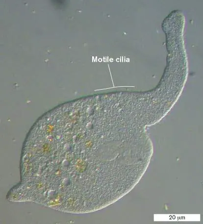
When we think of eukaryotes, we think first of plants and animals consisting of complex, multicellular bodies. But the domain Eukarya also contains vast numbers of microbes, including fungi as well as protists (algae and protozoa). Chapter 20 introduces the diverse kinds of eukaryotic microbes and their various niches in life on Earth. Fungi include unicellular yeasts and filamentous Penicillium. Algae conduct photosynthesis using chloroplasts; some form long sheets of seaweed, while others are single-celled phytoplankton. Protozoa are motile heterotrophs that include amebas, ciliates, and many types of parasites.
Protozoan parasites cause diseases such as malaria and sleeping sickness, but most protozoa in nature are free-living predators, as voracious as any animal. For example, the predator Lacrymaria olor, seen in the chapter-opening image, consists of a single cell full of cilia, tiny hairs that beat in waves. This cell extends a flexible neck with a “head” that hunts for prey. When it captures the prey, usually a smaller ciliate, it engulfs the cell into its cytoplasm.
Other kinds of protists are phototrophs that play vital roles in our oceans. A compelling example is the dinoflagellate family Symbiodiniaceae, whose species form endosymbioses with corals. The algal cells take up residence within the coral tissues, where their photosynthesis drives the growth of reefs that support vast ecosystems of marine life. The existence of corals worldwide is threatened by global climate change. Rising temperatures and acidity upset the delicate mutualism of coral and its algal partners, which must then either adapt or die.
20.1 Phylogeny of Eukaryotesnot assigned
Chapter 20 presents the phylogeny of major groups of microbial eukaryotes, along with the branching of animals and plants from the microbial family tree. We explore the form and function of algae, such as the calcium carbonate–plated coccolithophores that bloom over vast stretches of ocean (Fig. 20.1A). Fungi range from yeast to mushrooms to common molds such as Penicillium, our source of penicillin (Fig. 20.1B ). Protozoa include a dozen deep-branching clades, from free-living amebas to diarrhea-causing parasites such as Giardia (Fig. 20.1C ). We get to know the eukaryotic microbes as essential partners in ecosystems and as infectious agents that cause some devastating diseases.
FIGURE 20.1 ■ Microbial eukaryotes. A. Coccolithus pelagicus, a marine coccolithophore, single-celled alga that forms scales of calcium carbonate (colorized SEM). B.
Conidiophores of Penicillium notatum, an airborne fungus
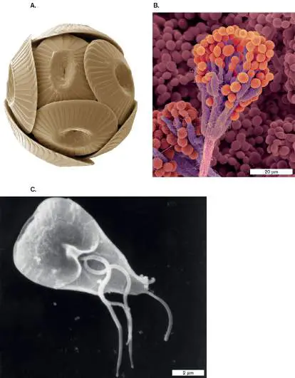
(colorized SEM). C. Giardia intestinalis, a waterborne parasite (SEM).
THE NATURAL HISTORY MUSEUM/ALAMY STOCK PHOTO
DENNIS KUNKEL MICROSCOPY/SCIENCE SOURCE
CDC/JANICE HANEY CARR
The Eukaryotic Cell
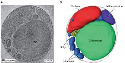
With all their diversity, eukaryotic cells share a common structure defined by the presence of the nucleus and other membrane-enclosed organelles (for review, see eAppendix 2). The extensive compartmentalization of the eukaryotic cell, including the nucleus and endomembrane system, enables eukaryotic cells to grow 1,000-fold larger than prokaryotic cells. Yet these organelles are found within even the tiniest of eukaryotes, such as Ostreococcus tauri, a green alga about 1 μm across (Fig. 20.2). This alga consists of a round, coccoid cell containing one or two of each major type of organelle—a mitochondrion, a chloroplast, and a stack of Golgi—all packed within the cell’s small volume. The genome of O. tauri is also downsized; at only 12 megabases (Mb), the genome is barely three times as long as that of the bacterium Escherichia coli. Though poorly understood, such tiny, bacteria-sized eukaryotes are believed to be the most numerous and ubiquitous forms of eukaryotic life. FIGURE 20.2 ■ A tiny eukaryote still has organelles. Ostreococcus tauri, visualized by cryo-electron microscopy (A) and in 3D by tomography (B) .
COURTESY OF GRANT JENSEN
DIARMUID/ALAMY STOCK PHOTO
Note that despite their extraordinary range of form, the metabolism of eukaryotes is less diverse than that of either bacteria or archaea. Most eukaryotes conduct either oxygenic photosynthesis or heterotrophy—or both. All have descended from an ancestral cell that engulfed a bacterial endosymbiont, giving rise to mitochondria, the source of aerobic respiration. And all eukaryotic phototrophs possess chloroplasts that descended from a cyanobacterial ancestor.
Historical Overview of Eukaryotes
For most of human history, life was understood in terms of macroscopic, multicellular eukaryotes: animals (creatures that move to obtain food) and plants (rooted organisms that grow in sunlight). Fungi (singular, fungus), which lack photosynthesis, were nonetheless considered a form of plant because they grow on the soil or other substrate. Thus, mycology, the study of fungi, was often included with botany, the study of plants. But the basis of
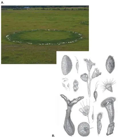
fungal growth was poorly understood, and its mystery was often associated with magic. For example, people were mystified by the sudden growth of mushrooms in a ring, which they called a “fairy ring” (Fig. 20.3A). The mushrooms actually arise as fruiting bodies from the tips of fungal hyphae (filaments of cells) that propagate from a single spore and extend radially underground.
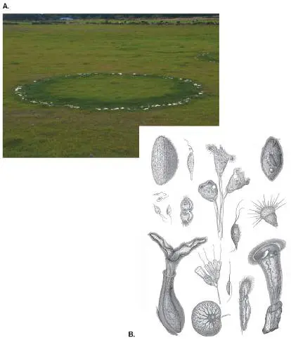
FIGURE 20.3 ■ Traditional views of fungi and protozoa (protists). A. Basidiomycete mushrooms growing in a “fairy ring.” B. A nineteenth-century depiction of various protozoa, by Rudolf Leuckart.
NASTASIC/GETTY IMAGES
In the eighteenth and nineteenth centuries, microscopists came to recognize microscopic forms of fungi such as filamentous hyphae and unicellular yeasts. Other unicellular life forms, such as amebas and paramecia, were motile and appeared more like microscopic animals. These animal-like organisms were called protozoa (singular, protozoan; Fig. 20.3B ). The cellular dimensions of protozoa were typically 10-to 100-fold larger than those of known bacteria, and their form and motility offered intriguing subjects for observation. So did single-celled phototrophs such as diatoms and dinoflagellates, which were called algae (singular, alga). Algae were thought of as unicellular plants, although simple multicellular algae were known. The unicellular and microscopic forms of fungi, protozoa, and algae came to be included in the subject of microbiology.
Discoveries in physiology led us to redefine these organisms. For example, some of the motile organisms defined as protozoa contain chloroplasts and are classified as secondary endosymbiont algae. On the other hand, slime molds, originally classified with fungi, show form and motility more typical of protozoa. By the mid-twentieth century, naturalists classified protozoa, unicellular algae, and undifferentiated colonial forms as protists. Researchers including Herbert Copeland, Robert Whittaker, and Lynn Margulis attempted to refine the definition of “protist” to better distinguish microbial life forms.
Today, molecular phylogeny shows that protists comprise several clades equally distant from each other as they are from animals and plants (Fig. 20.4). In the terminology used today: Protist refers to single-celled and colonial eukaryotes other than fungi. Protists include many diverse clades of algae and protozoa.
Protozoa are protists that are single-celled heterotrophs. They include environmental consumers, as well as medically important parasites such as Giardia.
The algae include two major kinds. Those of the first kind are derived from a single endosymbiotic event and are closely related to green plants. These algae are called primary algae (Plantae in Fig. 20.4). By contrast, various groups of heterotrophic protists later incorporated algae in a second event of symbiogenesis. These are secondary algae (green asterisks in Fig. 20.4).
FIGURE 20.4 ■ Eukaryotic phylogeny. A phylogenetic tree of major clades (supergroups) of eukaryotes based on DNA sequence data. Dotted lines denote uncertain lineage. Green
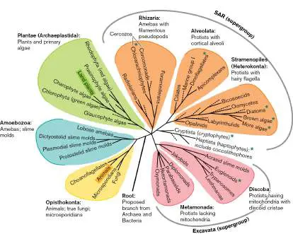
asterisks denote secondary algae whose ancestor engulfed a primary alga with chloroplast.
Sources: Modified from Sandra L. Baldauf. 2003. Science 300 :1703; and Fabien Burki et al. 2020. Trends Ecol. Evol. 35 :43.
Note: Medical textbooks also cover invertebrate animal parasites
such as worms and mites as eukaryotic agents of disease, although they are not considered microbes.
Challenges for Classification
Classifying eukaryotes presents several challenges. A major challenge for classification is the size and complexity of eukaryotic genomes. Eukaryotic genomes are typically severalfold larger than those of bacteria and archaea, and 50%–90% of their DNA consists of noncoding sequences. Thus, eukaryotic genomes take longer to sequence and are more challenging to annotate than those of prokaryotes.
As they evolve, microbial eukaryotes frequently lose structures through reductive (degenerative) evolution. Thus, for example, a clade originally defined by possession of flagella often includes members that lack flagella. In addition, superficially similar forms of organisms have evolved independently in distantly related taxa; this is called convergent evolution. For example, the “water molds” that grow on aquarium fish superficially resemble fungi, but they actually evolved in a clade that includes brown algae and diatoms. Many emerging clades consist of predatory protists with flagella or cilia that are distantly related to the well-known flagellates and ciliates such as alveolates and paramecia.
Furthermore, the evolution of eukaryotes includes multiple events of endosymbiosis, in which an engulfed cell evolved into an essential organelle. An endosymbiotic incorporation of a proteobacterium by the ancestor of all eukaryotes gave rise to mitochondria. Later, incorporation of a cyanobacterium by the ancestor of plants and algae gave rise to chloroplasts. Much later, several lineages of protists took up chloroplast-bearing algae, which now show varying stages of evolution as organelles.
The names and groupings of eukaryotic clades are changed as new evidence emerges. A current consensus view of eukaryotic phylogeny (Fig. 20.4) is based on phylogenomics, the comparison of whole genomes including thousands of protein-encoding sequences. Phylogenomics is conducted largely by computational analysis. Ultimately, the taxonomist builds a tree on the basis of maximum likelihood; that is, a tree of past divergence that appears the most probable on the basis of current data. As more data appear, inevitably the tree branches are refined.
We will now survey key traits of some major groups of taxa shown in Figure 20.4. In addition, Table 20.1summarizes traits of some representative clades.
Eukaryotic Microbial
TABLE 20.1
Diversity
Opisthokonta (fungi and metazoan animals). Single flagellum on reproductive cells. Includes multicellular animals.
Metazoa (animals). Multicellular organisms with motile body parts. Includes colonial animals, both invertebrates and vertebrates. Homo sapiens.
Choanoflagellata. Single flagellum and collar of microvilli. Resemble sponge choanocytes. Possible link to common ancestor of multicellular animals.
Eukaryotic Microbial
TABLE 20.1
Diversity
Cryptista. Unicellular biflagellar algae derived from secondary endosymbiosis.
Fungi (Eumycota). Cells form hyphae with cell walls of chitin.
Ascomycota. Fruiting bodies form asci containing haploid ascospores. Includes opportunistic pathogens and bread-making yeasts. Penicillium, Aspergillus, Saccharomyces cerevisiae, Stachybotrys. Lichens are a mutualism between an ascomycete and green algae ( Trebouxia) or cyanobacteria (Nostoc).
Basidiomycota. Basidiospores form primary and secondary mycelia; some generate mushrooms. May be edible (Lycoperdon) or toxic (Amanita). Plant pathogens (Ustilago maydis causes corn smut). Human pathogens (Cryptococcus neoformans).
Chytridiomycota. Motile zoospores with a single flagellum. Saprophytes or anaerobic rumen fungi. Allomyces. Frog pathogens (Batrachochytrium dendrobatidis). Bovine rumen digestive endosymbionts ( Neocallimastix).
Glomeromycota. Mutualists of plant roots, forming arbuscular mycorrhizae, filamentous networks that share nutrients with and among diverse plants.
Zygomycota. Sexual hyphae (haploid) grow toward each other and fuse to form the zygote (zygospore). Saprophytes or insect parasites.
Eukaryotic Microbial
TABLE 20.1
Diversity
Microsporidia. Single-celled parasites that inject a spore through a tube into a host cell, causing microsporidiosis. Encephalitozoon species. Commonly infect AIDS patients. Amoebozoa (amebas and slime molds). Lobe-shaped (lobose) pseudopods driven by sol-gel transition of actin filaments. Share branch with Opisthokonta.
Amebas. Unicellular. Life cycle is primarily asexual. Predators in soil or water. Giant free-living amebas (Amoeba proteus ); parasites (Entamoeba histolytica).
Mycetozoa. Slime molds. Cellular slime molds ( Dictyostelium). Upon starvation, amebas aggregate to form a fruiting body, which produces spores. Plasmodial slime molds (Physarum polycephalum) undergo meiosis, producing spores that germinate to form haploid amebas. Plantae or Archaeplastida (primary endosymbiotic algae and plants). Includes green algae and multicellular land plants. Chloroplasts all arose from a single cyanobacterial endosymbiont.
Chlorophyta (green algae). Green plastids contain chlorophylls a and b.
Unicellular with paired flagella. Chlamydomonas, Volvox (colonial).
Multicellular. Spirogyra grows in chains; Ulva grows in sheets; Cymopolia forms calcified stalks with filaments.
Eukaryotic Microbial
TABLE 20.1
Diversity
Glaucophyta. Unicellular algae whose chloroplasts have peptidoglycan.
Picoeukaryotes. Ostreococcus and Micromonas are unicellular algae.
Siphonous algae. Caulerpa species consist of a single cell with multiple nuclei, growing to indefinite size. Haptista (includes Haptophyta). Most are marine algae with outer scales; form large blooms.
Prymnesiophyceae. Coccolithophores. Possess calcified scales.
Rhodophyta (red algae). Phycoerythrin obscures chlorophyll, colors the algae red. Absorption of blue-green light enables colonization of deeper waters. Porphyra forms sheets edible by humans; Mesophyllum is a coralline alga, hardened by calcium carbonate crust; resembles coral. SAR (Stramenopiles, Alveolata, Rhizaria)
Stramenopiles (Heterokonta). Paired flagella of dissimilar form, one forward-pointing with hairs.
Bacillariophyceae. Diatoms.
Chrysophyceae. Golden algae.
Oomycetes. Water molds.
Phaeophyceae. Kelps.
Alveolata (having cortical alveoli). Cortex contains flattened vesicles called alveoli, reinforced below by lateral microtubules.
Apicomplexa (formerly Sporozoa). Parasites with complex life cycles. Lack flagella or cilia; possess apical complex for invasion of host cells. Vestigial chloroplasts.
Eukaryotic Microbial
TABLE 20.1
Diversity
Plasmodium falciparum causes malaria; Toxoplasma gondii causes feline-transmitted toxoplasmosis; Cryptosporidium parvum is a waterborne opportunistic parasite.
Ciliophora. Common aquatic predators. Undergo sexual exchange by conjugation, in which micronuclei are exchanged, then regenerate macronuclei. Covered with cilia (Paramecium); mouth ringed with cilia (Vorticella ); suctorians (Acineta).
Dinoflagellata. Secondary or tertiary endosymbiont algae, from engulfment of primary or secondary algae. Cortical alveoli contain stiff plates. Pair of flagella, one wrapped around the cell. Free-living aquatic (Peridinium ); zooxanthellae, endosymbionts of coral (Symbiodinium ).
Rhizaria (amebas with filament-shaped pseudopods). Filament-shaped (filose) pseudopods. Some species have a test (shell) of silica or other inorganic materials. Possess flagella or pseudopods (Cercozoa); form spiral tests (Foraminifera); form thin pseudopods called filopodia (Radiolaria).
Discoba (having disk-shaped cristae). Disk-shaped cristae of mitochondria. Parasitic or symbiotic flagellates; some alternate with ameboid forms. Euglena, Trypanosoma, Naegleria.
Metamonada (vestigial mitochondria). Parasitic or symbiotic flagellates. Mitochondria and Golgi degenerated through evolution. Includes human parasites Giardia and Trichomonas and symbionts of termite gut (Pyrsonympha).
Opisthokonts: Animals and Fungi
Where do humans and other multicellular animals fit into the eukaryotes? The position of animals (Metazoa) among the eukaryotic microbial clades is of interest because it suggests which contemporary microbes most closely resemble our own cells. The degree of relatedness can help define microbial model systems for probing key questions of human cell biology. For example, the baker’s yeast Saccharomyces cerevisiae shares enough of its genetic machinery with humans that it provides a model for cancer, defects in cellular trafficking, and degenerative brain disorders. The yeast S. cerevisiae is a fungus—and in fact, genomic analysis relates animals more closely to fungi (such as yeasts) than to motile microbial eukaryotes (such as paramecia or amebas). The true fungi, or Eumycota, are heterotrophs, either single-celled or growing in nonmotile filaments of cells called hyphae. Animal and fungal cells also share a structural feature distinguishing them from protists: the presence of an unpaired flagellum. Both animals and fungi include species whose life cycle has a uniflagellar stage, in contrast to many microbial eukaryotes whose flagella are paired, such as the parasite Giardia. In the case of humans, the uniflagellar stage is the spermatozoan. Similarly, some species of fungi generate uniflagellar reproductive cells called zoospores. As a whole, the clade including single-flagellum members is termed “opisthokont,” based on the Greek words meaning “backward-pointing pole,” because the flagellum points backward like an oar.
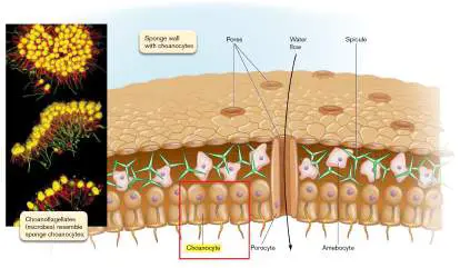
Among opisthokonts, the microbes that diverged from animals most recently (600 million years ago) appear to be the choanoflagellates. Genetic studies of choanoflagellates reveal several genes found only in animals. The prefix “choano-” (meaning “funnel”) refers to the collar of filaments surrounding the flagellum. The collared cells of choanoflagellates closely resemble the choanocyte cells of colonial sponges, an ancient form of animal ( Fig. 20.5). In 2019, Nicole King and colleagues at UC Berkeley showed that some choanoflagellates can assemble in a cuplike colony that undergoes coordinated movement, like an animal tissue. Thus, choanoflagellates may represent a “missing link” between animals and the microbial eukaryotes.
FIGURE 20.5 ■ Choanoflagellates resemble sponge choanocytes. Sponge choanocytes resemble choanoflagellates. Within the sponge, choanocytes assist the circulation of water and the uptake of nutrients. Inset: Choanoflagellates, single-celled microbes that form colonies resembling an animal cell layer.
Source: Nicole King.
THIBAUT BRUNET (HOWARD HUGHES MEDICAL INSTITUTE/UNIVERSITY OF
CALIFORNIA BERKELEY)
Note: Eukaryotic flagella are whiplike organelles composed of
microtubules and surrounded by a membrane; their action is powered by ATP along the entire filament. Distinguish them from bacterial and archaeal flagella, which are rotary, helical filaments
composed entirely of protein subunits; their rotation is powered at the base by proton motive force.
Thought Question
20.1 How could you demonstrate that eukaryotic flagella move with a whiplike motion instead of rotary motion? What experiment might you conduct?
Several taxa that historically were grouped with fungi (for example, slime molds) are now classified in more deeply branching clades of protists. Slime molds generate populations of cells that migrate into a unified structure called a fruiting body to make reproductive cells. Slime molds are now grouped with amebas (supergroup Amoebozoa; discussed in Section 20.3). Water molds, which are plant and animal pathogens of the class Oomycetes (supergroup SAR, Stramenopiles), are now recognized as heterokont protists.
Amoebozoa Branch Near Opisthokonts but Far from Rhizaria
Amebas (also spelled amoebas ) are unicellular organisms of highly variable shape that form pseudopods, locomotory extensions of cytoplasm enclosed by the cell membrane. Their size can reach several millimeters, and they can eat small invertebrate animals. The Amoebozoa, the most familiar kind of amebas, have lobed pseudopods, pseudopods that extend lobes of cytoplasm through cytoplasmic streaming. Most lobed amebas are free-living in aquatic habitats, but some cause human diseases such as amebic dysentery. Still other kinds of lobed amebas are cellular slime molds, in which individual amebas converge to form a fruiting body.
A more deeply branching group of protists that were historically called “amebas” is the Rhizaria (Table 20.1). The Rhizaria actually branch in the SAR supergroup (Stramenopiles, Alveolata, Rhizaria). Rhizaria have thin, filamentous pseudopods, often radially arranged like a star, as in heliozoa. Some Rhizaria, such as the foraminiferans, form inorganic shells called tests. Fossil foraminiferan tests are common in rock formations derived from ancient seas. Foraminiferan shells can be found in the White Cliffs of Dover in Britain and in the stone used to build the Egyptian pyramids.
Algae Evolved by Engulfing Phototrophs
Algae are commonly defined as single-celled plants and simple multicellular plants lacking true stems, roots, and leaves. Algal cells contain chloroplasts, membrane-enclosed organelles of photosynthesis that evolved from a cyanobacterium (Fig. 20.6). In Earth’s biosphere, algae plus bacterial phototrophs feed all marine and freshwater ecosystems, producing the majority of oxygen and biomass available for Earth’s consumers.
FIGURE 20.6 ■ Chloroplast evolution: primary and secondary endosymbiosis. A. Green algae (Chlorophyta) and red algae (Rhodophyta) contain chloroplasts (green) that evolved from engulfed cyanobacteria. B. Cryptophyte (cryptomonad) algae contain chloroplasts (green); cryptophyte
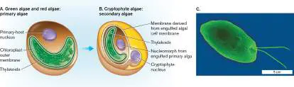
secondary-host cytoplasm (yellow); and a vestigial nucleus, or nucleomorph (purple), from the engulfed primary endosymbiont. C. Marine cryptomonad, Rhodomonas salina (colorized SEM), shows double flagella.
DENNIS KUNKEL MICROSCOPY/SCIENCE SOURCE
How did ancestral algae get their chloroplasts? The Plantae (Archaeplastida) include the primary algae and land plants, all of which descended from a common ancestor containing a chloroplast. The chloroplast evolved by endosymbiosis between an ancient protist and a cyanobacterium (discussed in Chapter 17). In primary algae, the chloroplast is enclosed by two membranes (Fig. 20.6A ): the inner membrane (from the ancestral phototroph’s cell membrane) and the outer membrane (from the host cell membrane as it enclosed its prey). Both green algae (chlorophytes) and red algae (rhodophytes) are primary algae. Their chloroplasts diverged from their common ancestor to use pigments absorbing different ranges of the light spectrum.
Surprisingly, several other taxa traditionally called algae evolved through a secondary endosymbiosis with a second protist host. The protist that engulfed the primary alga was usually a predatory protozoan. Nevertheless, the resulting organisms are called secondary algae. The symbiotic history of these secondary algae is most evident in the cryptophytes (Fig. 20.6B ), which still retain a vestigial nucleus, or nucleomorph, derived from the engulfed alga. In secondary algae, the chloroplast is surrounded by two extra membranes—one from the primary alga and one from the secondary host. An example of a secondary alga, the cryptomonad Rhodomonas salina, is shown in Figure 20.6C . This cryptomonad is now classed in the Cryptista supergroup (Fig. 20.4).
Cryptomonads and other secondary algae are abundant in the oceans. Other secondary algae include kelps and diatoms (supergroup SAR, Stramenopiles). The dinoflagellates (supergroup SAR, Alveolata) are secondary or tertiary algae, descended from a flagellate that consumed one or more types of algae. Dinoflagellates also engage in “kleptoplasty,” or “chloroplast stealing,” in which the chloroplast of a digested prey is retained long enough to derive some photosynthetic energy, but ultimately consumed. The variety of endosymbiosis among protists provides clues as to how the original chloroplast evolved within the ancestral algae.
Note: “Algae” may refer to primary endosymbiont algae, as well
as secondary algae that derive from deeply branching clades of protists. “Primary algae” comprise a monophyletic clade, all of whose members descend from one product of endosymbiosis that evolved the chloroplast. “Algae” and “secondary algae” are polyphyletic terms that include various lineages that derive from secondary engulfments by different predatory protozoa.
Other Protist Clades
Protists include multiple distantly related categories of eukaryotes (see Fig. 20.4and Table 20.1). Aside from algae, all protists are heterotrophs, commonly predators or parasites, although some such as dinoflagellates also conduct photosynthesis as secondary algae. Protists are important producers and consumers in marine, freshwater, and soil food webs. In ecology, phototrophic protists are termed “phytoplankton” and heterotrophs are termed “zooplankton,” although many, in fact, are “mixotrophs” that act as both producers and consumers.
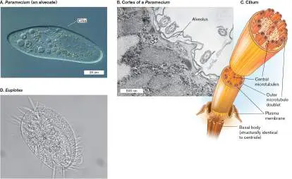
Alveolates (supergroup SAR, Alveolata) include ciliated protists (ciliates), dinoflagellates, and apicomplexans. An example is the ciliate Paramecium (Fig. 20.7A). Alveolates are known for their complex outer covering, or cortex. The cortex contains networks of vesicles just under the cell membrane, called cortical alveoli (singular, alveolus ) (Fig. 20.7B ). Alveoli store calcium ions, and in some species protective plates form within them. Organisms equipped with paired flagella or cilia are known as flagellates and ciliates, respectively. Flagella (singular, flagellum ) and cilia (singular, cilium) are essentially equivalent organelles composed of microtubules and enveloped by the cell membrane (Fig. 20.7C ). Cilia are shorter than most flagella and more numerous, and usually are distributed over a broad surface of the cell. For example, the motile ciliate Euplotes possesses rows of cilia that beat in waves of coordinated motion (Fig. 20.7D ).
FIGURE 20.7 ■ The cortex of an alveolate contains alveoli. A. The alveolate Paramecium is covered with cilia. B. Cortex of Paramecium tetraurelia with alveoli (thin section, TEM). C. A cilium is composed of doublet microtubules enveloped in cell membrane. Flagella are similar in structure but can be much longer. D. Euplotes demonstrates ciliary motion.
Source: Part D from Danxu Tang et al. 2020. Front. Microbiol. 11 :549781.
M. I. WALKER/SCIENCE SOURCE
RICHARD ALLEN (UNIVERSITY OF HAWAII) (2011)
D. TANG ET AL. 2020. FRONT MICROBIOL. 11 :549781
Alveolata also includes a major group of parasites, most of which lack flagella, the apicomplexans. A well-known apicomplexan
parasite is Plasmodium falciparum, which causes malaria.
Stramenopiles (under supergroup SAR) possess pairs of different-length flagella at some point in the life cycle, with one forward-pointing flagellum having long stiff hairs (Table 20.1). This trait distinguishes stramenopiles from opisthokonts, which possess a single hairless flagellum (if any). Flagellated stramenopiles include voracious zooplankton, common in marine and freshwater environments.
The Discoba include free-living protists such as euglenas, as well as parasites showing extensive evolutionary reduction. Most Discoba have mitochondria with distinctive disk-shaped cristae (membrane pockets). Parasitic Discoba include the trypanosomatids that cause sleeping sickness and Chagas’ disease. A possibly related clade, Metamonada, includes the waterborne parasite Giardia intestinalis (also known as G. lamblia). In metamonads, the mitochondria have lost their genomes and degenerated (discussed in Section 20.6). Throughout the phylogenetic tree, various flagellates, ciliates, and ameboid protozoa show genomes deeply branching from more well-studied organisms. These include, for example, the clades Haptista and Cryptista as shown in Figure 20.4.
Emerging Eukaryotes
Are there still eukaryotes that we have yet to discover? Genes from natural communities continually reveal new species of microbial eukaryotes in previously unknown divisions. Many of the new isolates are single cells as small as bacteria, designated nanoeukaryotes (3–20 μm) and picoeukaryotes (0.2–3 μm).
Genetic analysis shows that similar miniaturized eukaryotes branch deeply from all groups in the phylogenetic tree, potentially doubling the known number of eukaryotic taxa. Furthermore, our metagenomic analysis reveals eukaryotes in environments previously believed to be restricted to bacteria and archaea, such as anaerobic submarine sediments and the hyperacidic Tinto River in Spain. In every new habitat tested, new deep-branching clades of eukaryotes emerge, with new implications for ecology and global cycling of elements (discussed in Chapters 21 and 22). The wealth of new genomic data continues to reshape our understanding of the domain Eukarya.
To Summarize
Opisthokonta includes true fungi (Eumycota) and multicellular animals (Metazoa), as well as related clades such as Microsporidia and choanoflagellates.
Plantae (Archaeplastida) includes primary algae and land plants. Secondary algae include various clades that independently evolved from secondary endosymbiosis between a predatory protozoan and a primary alga.
Predatory protist clades include Amoebozoa, amebas with lobe-shaped pseudopods; Rhizaria, including amebas with fine pseudopods; Alveolata, ciliates, flagellates, and parasites with complex cortical structure; Stramenopiles, the kelps, diatoms, and flagellates with nonequivalent paired flagella; and Discoba and Metamonada, primarily parasites.
Many protists are phototrophs as well as heterotrophs on the basis of secondary or tertiary endosymbiosis derived from engulfed algae.
Environmental sequence analysis continually reveals new clades of microbial eukaryotes. New kinds of microbial eukaryotes emerge from all habitats.
Glossary
fungus pl. fungi A heterotrophic opisthokont eukaryote with chitinous cell walls. Includes Eumycota, but traditionally may refer to fungus-like protists such as the oomycetes.
mycology The study of fungi.
protozoan pl. protozoa A heterotrophic eukaryotic microbe, usually motile, that is not a fungus.
protist A single-celled eukaryotic microbe, usually motile; not a fungus. primary algae Algae that are derived from a single endosymbiotic event; closely related to green plants (Plantae).
primary algae Algae that are derived from a single endosymbiotic event; closely related to green plants (Plantae).
secondary algae Algae that evolved by engulfing primary algae in a second endosymbiotic event.
secondary algae Algae that evolved by engulfing primary algae in a second endosymbiotic event.
endosymbiosis An intimate association between different species in which one partner population grows within the body of another organism. phylogenomics The construction of phylogenetic trees of related clades on the basis of comparison of whole genomes.
true fungi See Eumycota .
Eumycota True fungi, a taxonomic group of opisthokont eukaryotes with chitinous cell walls; the group most closely related to animals. zoospore A flagellated reproductive cell produced by chytridiomycete fungi.
fruiting body A multicellular fungal or bacterial reproductive structure. ameba or amoeba A protist that moves via pseudopods.
pseudopod A locomotory extension of cytoplasm enclosed by the cell membrane.
Rhizaria A clade of eukaryotic microbes that have filamentous pseudopods.
alga pl. algae A microbial eukaryote that contains chloroplasts.
alga pl. algae A microbial eukaryote that contains chloroplasts.
chloroplast An organelle of endosymbiotic origin (sharing descent with cyanobacteria) that conducts oxygenic photosynthesis; found in algae and plant cells.
Plantae Also called Archaeplastida. A eukaryotic superphylum that includes plants, as well as green and red primary algae. green alga Also called chlorophyte. A member of the eukaryotic group Chlorophyta—microbes that have chloroplasts; closely related to plants (Plantae).
chlorophyte See green alga .
red alga Also called rhodophyte. An alga of the eukaryotic group Rhodophyta, which contain chloroplasts as primary algae, with red accessory photopigments.
rhodophyte See red alga .
nucleomorph A vestigial nucleus within a eukaryotic cell, evolved by genetic reduction from the nucleus of an endosymbiont.
20.2 Funginot assigned
Fungi (Eumycota, under Opisthokonta) provide essential support for all communities of
multicellular organisms. Fungi recycle the biomass of wood and leaves, including
substances such as lignin, which other organisms may be unable to digest. Underground
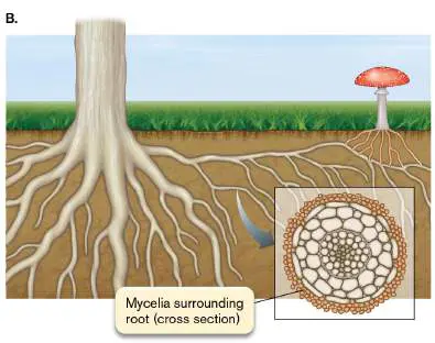
fungal filaments called mycorrhizae extend the root systems of most plants, forming a
nutritional “Internet” that interconnects the plant community (discussed in Chapter 21).
Mycorrhizae may have inspired the fictional underground tree network depicted in the
film Avatar (2009).
Within the ruminant digestive tract, fungi ferment plant materials. On the other
hand, pathogenic fungi infect plants and animals, and they contribute to the death of
immunocompromised human patients. Still other fungi produce antibiotics such as
penicillin, as well as food products such as wine and cheeses (discussed in Chapter 16).
Shared Traits of Fungi
Most fungi share these distinctive traits:
Absorptive nutrition. Most fungi cannot ingest particulate food, as do protists,
because their cell walls cannot part and re-form, as do the flexible pellicles of
amebas and ciliates. Instead they secrete digestive enzymes and then absorb the
broken-down molecules from their environment.
Hyphae. Most fungi grow by extending multinucleate cellular filaments called
hyphae (singular, hypha; Fig. 20.8A ). As a hypha extends, its nuclei divide
mitotically without cell division, generating a multinucleate cell. Later, septa may
form to partition the hypha into cells. Hyphae grow by cytoplasmic extension and
branching. A branched mass of extending hyphae is called a mycelium (plural,
mycelia). Figure 20.8B shows hyphal growth of Mucor circinelloides, a human
pathogenic zygomycete.
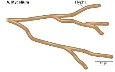
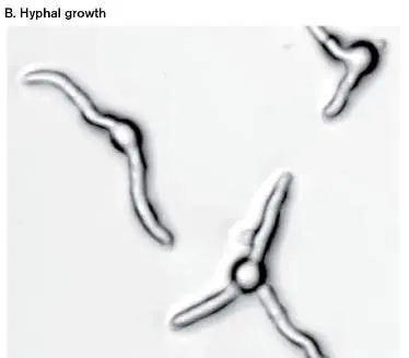
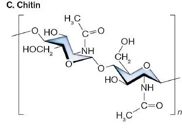
FIGURE 20.8 ■ Fungi grow hyphae with cell walls of chitin. A. Fungal
hyphae extend and form branches, generating a mycelium. B. Hyphae grow
into mycelia in Mucor circinelloides. C. Chitin consists of beta-1,4-linked N-
acetyl-D-glucosamine. Source: Part B from Soo Chan Lee et al. 2013. PloS
Pathog. 9 :e1003625.
S. C. LEE ET AL. 2013. PLOS PATHOG. 9 :E1003625
Cell walls contain chitin. Chitin is an acetylated amino-polysaccharide of
immense tensile strength, stronger than steel (Fig. 20.8C ). Its strength derives
from multiple hydrogen bonds between fibers. Chitinous cell walls enable fungi to
penetrate plant or animal cells, including tough materials such as wood. Inhibitors
of chitin synthesis, such as the polyoxins and nikkomycins, are used as antibiotics
against fungal infections.
Membranes contain ergosterol. Ergosterol is an analog of cholesterol not found
in animals or plants. Ergosterol is so distinctive to fungi that its presence can be
used as a measure of fungal content in plant food products such as grains.
Inhibitors of ergosterol biosynthesis, such as the triazoles, are used to treat fungal
infections. Another antifungal agent, nystatin, specifically binds ergosterol and
forms membrane pores that leak K + ions.
Fungal Hyphae Absorb Nutrients
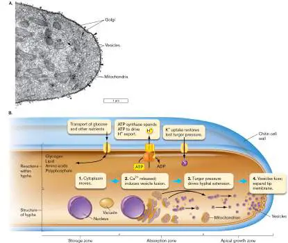
How do fungal hyphae grow and form colonies of “mold”? A fungal hypha expands at
the tip. Cytoplasmic expansion is driven by turgor pressure against the chitin cell wall—
the force that enables fungi to penetrate tough materials such as wood. Fungal hyphae
can extend as fast as half a centimeter per hour.
The cytoplasmic turgor pressure is regulated by uptake of hydrogen ions in exchange
for potassium ions (Fig. 20.9 ). Loss of turgor pressure—for example, by puncture of
the hypha—leads to accelerated K + uptake and water influx, restoring turgor. Molecules
that cause loss of K +, such as nystatin, serve as antifungal agents.
FIGURE 20.9 ■ Cellular basis of hyphal extension. A. Section through the
growing tip of a hypha (TEM). Vesicles collect at the tip, where they fuse into the
cell membrane, enabling extension. B. The absorption zone takes in nutrients.
Cytoplasm moves toward the tip of the apical growth zone, driven by turgor
pressure. Turgor pressure is regulated by H + export and K + uptake. Ca 2+ released
by the endoplasmic reticulum and mitochondria induces vesicles to fuse and to
expand the plasma membrane at the growing tip.
STEPHEN SEILER ET AL. 1997. EMBO J. 16 :3025–3034, FIG. 8A
At the hypha’s growing tip, turgor pressure pushes the cell membrane forward, and
the membrane expands by incorporating vesicles generated from the endoplasmic
reticulum (as seen in Fig. 20.9A ). The endoplasmic reticulum and mitochondria store
Ca 2+, whose release triggers vesicle fusion with the plasma membrane. The fused
vesicles provide phospholipids and proteins to extend the membrane surface area as
the cytoplasm expands.
Just behind the hypha’s growing tip lies its absorption zone (Fig. 20.9B ). The
absorption zone takes in nutrients from the surrounding medium, such as the cytoplasm
of an invaded animal cell. Behind the absorption zone, the older part of the hypha
collects and stores nutrients. As the storage zone expands, the nucleus divides multiple
times. Septa form across the hypha, partly compartmentalizing the cytoplasm. As the
older part of the hypha ages, its tubular form begins to lyse, releasing cell contents.
This aging part of the hypha is called the senescence zone (not shown in the figure).
As hyphae grow, branches extend from their sides. The hyphae branch and extend
radially, forming the mycelium. The mycelium forms the characteristic round, fuzzy
colony of a fungus or “mold.” On a substrate such as wood or agar, mycelia grow in two
forms: aerial mycelium, which extends out into the air; and surface mycelium, which
grows into and along the surface of the substrate.
Unicellular Fungi
Despite the advantages of multinucleate hyphae, some fungi are unicellular,
known as yeasts. Yeast forms evolved in many different fungal taxa. The yeast
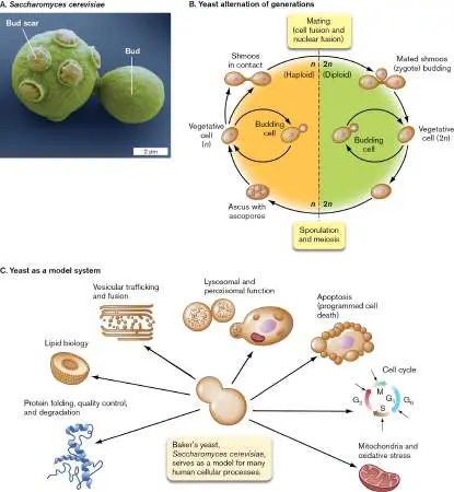
Saccharomyces cerevisiae (Fig. 20.10A ) is used to make bread rise and to
brew wine and beer (for more on food microbiology, see Chapter 16). S. cerevisiae
reproduces by budding, in which mitosis of the mother cell generates daughter cells of
smaller size. The mother cell acquires a bud scar where the smaller one pinched off (
Fig. 20.10A ). After generating a limited number of buds, the mother cell senesces and
dies. Thus, yeasts provide a unicellular model system for the process of aging.
FIGURE 20.10 ■ Yeasts are nonmycelial fungi. A. Saccharomyces cerevisiae
, or baker’s yeast, reproduces by budding (colorized SEM). Upper cell shows six bud
scars. B. In the life cycle of S. cerevisiae, haploid cells reproduce many generations
by budding. C. S. cerevisiae serves as a model for human cellular processes.
Source: Part C modified from Vikram Khurana and Susan Lindquist. 2010. Nat. Rev. Neurosci. 11
:436–449.
EYE OF SCIENCE/SCIENCE SOURCE
Other yeasts, such as Candida albicans, are important members of the human
vaginal microbiome but can cause opportunistic infections. Some are important
opportunistic pathogens, occurring frequently in AIDS patients; for example,
Pneumocystis jirovecii (formerly P. carinii) is a yeast-form ascomycete, whereas
Cryptococcus neoformans is a yeast-form basidiomycete (discussed shortly).
Pathogens such as Candida albicans can grow either as single cells (yeast form) or
as mycelia; because they exist in two different forms, these are known as “dimorphic”
fungi. The yeast form grows normally in the mucosa, but germination of mycelia leads
to disease. A very different dimorphic fungal pathogen is Blastomyces dermatitidis, the
cause of blastomycosis, a type of pneumonia. B. dermatitidis forms a mycelium in
culture and in soil environments, but it grows as a yeast within the infected lung.
Yeast as a model organism for research. The yeast Saccharomyces cerevisiae is a
model organism for research in eukaryotic biology (Fig. 20.10C ). Its cells grow
rapidly, in haploid and diploid forms, and are amenable to genetic recombination and
transformation. The yeast genome of 6,000 genes includes many human homologs,
such as the ras proto-oncogene (a gene involved in cancer). Often, entire networks of
proteins interacting in yeast have human homologs; thus, S. cerevisiae has been called
a “single-celled human.” Susan Lindquist (1949–2016) at MIT’s Whitehead Institute for
Biomedical Research developed yeast as a model for brain neuronal diseases such as
Alzheimer’s (Special Topic 20).
SPECIAL TOPIC 20 Yeast: A Single-Celled Human Brain
The yeast Saccharomyces cerevisiae provides a model for human diseases such as
cancer because it shares so many homologs of our genes. Most of these genes
encode fundamental parts of cells, such as actin and cell growth regulators. But, of
course, the single-celled fungus lacks the differentiated parts and connectors of
human cells such as neurons. So, yeast could not serve as a model for complex
diseases of the brain. Or could it? What sounds impossible was accomplished by
the pioneering yeast molecular biologist Susan Lindquist (1949–2016) at the
Whitehead Institute for Biomedical Research (Fig. ST 20.1 ). An extraordinary
molecular biologist, Lindquist earned the National Medal of Science in 2010, and
she was elected as a Foreign Member of the Royal Society of London in 2015.
FIGURE ST 20.1 ■ Susan Lindquist developed yeast models of
human disease.
SHUTTERSTOCK
Neurodegenerative diseases such as Alzheimer’s can result from disorders of
cell function, such as lysosomal storage and degradation. A possible cause is that a
protein called beta-amyloid gets cleaved to a peptide that is secreted; the
secreted peptide returns to the cell by endocytosis. The endocytosed beta-amyloid
peptide then interferes with intracellular trafficking by an unknown mechanism. To
investigate the mechanism of beta-amyloid toxicity, Lindquist developed a yeast
model.
First, she and her students constructed a yeast strain that expresses beta-
amyloid peptide from a plasmid. In this yeast strain the beta-amyloid gets
secreted, but it returns by endocytosis to the endoplasmic reticulum (ER) for
trafficking—just as it does in a human cell. So, what happens to the yeast? The
yeast grows more slowly because beta-amyloid disrupts ER trafficking.
The disruption of trafficking by beta-amyloid was consistent with its proposed
role in Alzheimer’s disease. But to strengthen the connection—and to reveal other
parts of the process—Lindquist used her yeast model to screen for yeast proteins
that could overcome beta-amyloid interference. So she transformed her yeast
model strain with a library of yeast genes that were “overexpressed” (that is,

expressed on a plasmid at levels severalfold greater than normal). She identified
23 suppressors, genes whose overexpression suppressed the effect of beta-
amyloid and restored normal yeast growth. The suppressors also restored normal
trafficking of a reporter protein, a fluorescent YFP fusion protein expressed by the
yeast genome (Fig. ST 20.2 ). The control cells showed reporter protein
fluorescence localized normally to the vacuole (Fig. ST 20.2A ). Beta-amyloid
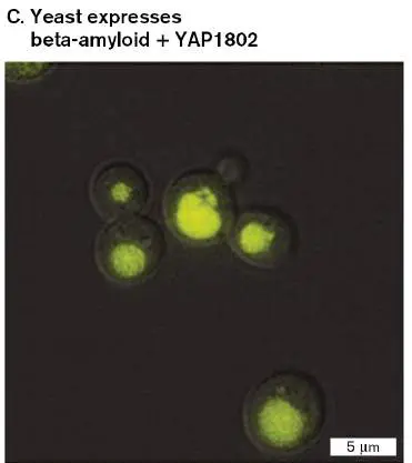
expression prevented trafficking to the vacuole (Fig. ST 20.2B ), but expression
of the suppressor protein YAP1802 restored movement to the vacuole (Fig. ST
20.2C ).
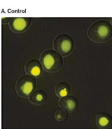
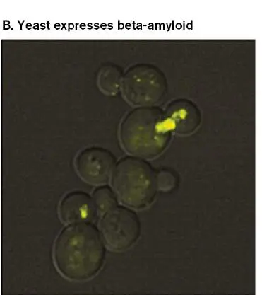
FIGURE ST 20.2 ■ Beta-amyloid disrupts traffic of yeast protein. A.
A yeast protein fused to yellow fluorescent protein (YFP) is trafficked normally
to the vacuole (fluorescence microscopy). B. Beta-amyloid expression
interferes with transport. C. YAP1802 expression restores transport.
SEBASTIAN TREUSCH ET AL. 2011. SCIENCE 334 :1241
SEBASTIAN TREUSCH ET AL. 2011. SCIENCE 334 :1241
SEBASTIAN TREUSCH ET AL. 2011. SCIENCE 334 :1241
At the time of her death in 2016, Lindquist was using the yeast model to
explore the mechanism of beta-amyloid’s effects within the cell and test possible
therapeutic agents for neurodegeneration. Her approach was picked up by
numerous colleagues, including Dina Petranovic at the Chalmers University of
Technology, Gothenburg, Sweden (Fig. ST 20.3A ). Petranovic developed a
“humanized” yeast beta-amyloid model that more closely resembles human cells in
the timing of expression of the toxic protein. Her model reveals several processes
that impact cell metabolism and morphology. Figure ST 20.3B and C shows the
visualization of yeast mitochondria, using two-photon excitation fluorescence
(TPEF), a method in which two infrared photons simultaneously excite the
fluorophore; this method achieves higher spatial resolution than does standard
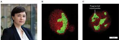
fluorescence. Yeast expressing beta-amyloids show fragmented mitochondria,
while respiration is decreased. This pathology resembles that seen in the brains of
Alzheimer’s patients. Petranovic dedicated her publication to the memory of Susan
Lindquist.
FIGURE ST 20.3 ■ Human beta-amyloid expression alters yeast
mitochondria. A. Dina Petranovic. B. Yeast control with mitochondria stained
green by rhodamine 123, viewed by two-photon excitation fluorescence (TPEF)
microscopy. C. Yeast expressing beta-amyloid oligomer show fragmented
mitochondria.
PHOTO BY JAN-OLOF YXELL, CHALMERS UNIVERSITY OF TECHNOLOGY
CAPTURED BY DR. NISHA AGARWAL. X. CHEN ET AL. 2017. FRONT. MOL. NEUROSCI. 10 :232
CAPTURED BY DR. NISHA AGARWAL. X. CHEN ET AL. 2017. FRONT. MOL. NEUROSCI. 10 :232
RESEARCH QUESTION
How would you use the humanized yeast model to identify therapeutic agents for
Alzheimer’s disease?
Treusch, Sebastian, Shusei Hamamichi, Jessica L. Goodman, Kent E. S. Matlack, Chee
Yeun Chung, et al. 2011. Functional links between Ab toxicity, endocytic trafficking, and
Alzheimer’s disease risk factors in yeast. Science 334 :1241–1245.
Chen, Xin, Markus M. M. Bisschops, Nisha R. Agarwal, Boyang Ji, Kumaravel P.
Shanmugavel, et al. 2017. Interplay of energetics and ER stress exacerbates Alzheimer’s
amyloid-β (Aβ) toxicity in yeast. Frontiers in Molecular Neuroscience 10 :232.
Thought Question
20.2 Why would yeasts remain unicellular? What are the relative advantages and
limitations of hyphae?
Yeast reproductive cycles. Some yeasts are asexual, whereas others can undergo
sexual alternation of generations (Fig. 20.10B ). This life cycle alternates between
generation of a haploid population, with a single copy of each chromosome (n), and a
diploid population, with a diploid chromosome number (2 n). The haploid form
develops gametes to fertilize each other, making a 2 n zygote. After vegetative
(nonsexual) divisions, the 2 n form undergoes meiosis, regenerating the haploid form.
(The process of meiosis is reviewed in eAppendix 2.) Alternation of generations allows
an organism to take advantage of favorable conditions by rapid asexual reproduction,
and to then respond to environmental change by reassorting its genes through meiosis
and by recombining them through fertilization. Gene reassortment and recombination
provide new genotypes, some of which may increase survival in the changed
environment.
In baker’s yeast (Saccharomyces cerevisiae), haploid spores divide and proliferate
by mitosis. Mating factors induce the haploid cells to differentiate into gamete forms
called “shmoos” (Fig. 20.10B ). Gametes of two different mating types fuse, and their
nuclei combine to form a zygote. In the diploid generation, the zygote divides
mitotically, generating a population of diploids that appear superficially similar to
haploid cells. Under starvation stress, the diploids undergo meiosis. Meiosis enables
cells to reassort their genes for combinations that may better survive the changed
environment. Meiosis generates an ascus (plural, sasci) that contains four haploid
spores.
Many fungi and protists undergo modified versions of alternation of generations,
utilizing a wide variety of haploid and diploid structures to accomplish essentially the
same genetic tasks. In many fungi, the haploid form predominates; for example,
ascomycetes such as Aspergillus and Neurospora form mainly haploid mycelia. In some
fungi, no sexual reproduction has been observed, probably because the inducing
conditions are unknown. Species that lack a known sexual cycle are called mitosporic
fungi, also known as “imperfect fungi.” Mitosporic species are found in many different
clades. An example is the famous Penicillium mold, an ascomycete, from which we
discovered the antibiotic penicillin.
Thought Question
20.3 Why would some fungi avoid sexual reproduction? What are the advantages and
limitations of sexual reproduction?
Mycelia, Mushrooms, and Mycorrhizae
Different species of fungi show vastly different forms, from the familiar mushrooms
(fruiting bodies that can weigh several pounds) to the mycelia of pathogens and the
symbiotic partners of algae in lichens. Major clades of fungi include Chytridiomycota,
Zygomycota, Ascomycota, and Basidiomycota.
Note: The major groups of fungi are also known by informal names with the
alternative suffix “-etes”: chytridiomycetes, zygomycetes, ascomycetes, basidiomycetes.
Chytridiomycota: motile zoospores with a single flagellum. The deepest-
branching group of fungi is Chytridiomycota (the chytridiomycetes, or chytrids), which
possess motile, flagellated reproductive forms called zoospores. In the chytrid taxa that
are well characterized, each zoospore possesses a single flagellum that points backward
as it propels the cell forward. The zoospore form has been lost by other fungi.
Chytrid species include bovine rumen inhabitants whose hyphae penetrate
tough plant material, facilitating digestion. Other chytrids are aerobic animal
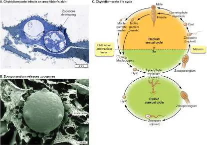
pathogens. Figure 20.11A shows the skin of a frog infected by the
chytridiomycete Batrachochytrium dendrobatidis. B. dendrobatidis has caused a
widespread die-off of frogs in Central and South America, in an epidemic associated
with global warming. The mycelium of B. dendrobatidis grows within the frog skin,
producing capsules full of diploid zoospores called zoosporangia. Each zoosporangium
protrudes through the skin surface, ready to expel zoospores in search of a new host (
Fig. 20.11B ).
FIGURE 20.11 ■ Chytridiomycete form and life cycle. A. A pathogenic
chytrid, Batrachochytrium dendrobatidis, infects the skin of an amphibian.
Amphibian skin cells are penetrated by discharge tubes of diploid zoosporangia
about to release zoospores. B. Zoosporangium releasing zoospores. C. Life cycle of
a chytrid. The diploid mycelium produces motile zoospores that form cysts in a poor
environment. Alternatively, the diploid mycelium undergoes meiosis to form a
haploid mycelium (gametophyte) that produces motile gametes.
DR. ELIZABETH DAVIDSON/VISUALS UNLIMITED, INC.
DR. ALEX HYATT, CSIRO AUSTRALIAN ANIMAL HEALTH LABORATORY
The life cycle of a chytrid includes mycelia that are haploid (gametophyte) or diploid
(sporophyte; Fig. 20.11C ). Haploid mycelia produce motile gametes that detect each
other by sex-specific attractants. The gametes fuse to produce a motile zygote. The
zygote forms a cyst, a cell with arrested metabolism that can persist for long periods. In
a favorable environment, the cyst germinates to form a diploid mycelium, or
sporophyte. The sporophyte generates zoosporangia full of zoospores. There are two
alternative forms of zoosporangia: those that produce diploid zoospores, which form
cysts and regenerate the diploid mycelium; and those that undergo meiosis to produce
haploid zoospores. The haploid zoospores generate a haploid mycelium (gametophyte)
capable of producing haploid gametes.
Zygomycota: nonmotile sporangia. The zygomycetes and other nonchytridiomycete
fungi generate nonmotile spores. Nonmotile spores require transport by air or water or
ballistic expulsion (expulsion under pressure) from a spore-bearing organ, called the
sporangium (plural, sporangia). A common zygomycete is the bread mold Rhizopus (
Fig. 20.12A ). Most zygomycetes, such as Mucor species, are soil molds that
decompose plant material or other fungi or the droppings of animals (Fig. 20.12B ).
These modest molds fill important niches in all terrestrial ecosystems.
FIGURE 20.12 ■ Zygomycete fungi form nonmotile sporangia. A. Rhizopus
(bread mold) haploid sporangia contain sporangiospores. B. Diploid hyphae of
Mucor species terminate in zygospores. C. The life cycle of zygomycetes involves
primarily haploid mycelia. Special hyphae form gametes at their tips. Gametes of
different mating types fuse to form the diploid zygospore. The zygospore undergoes
meiosis, regenerating haploid cells that form sporangia. The sporangia release
sporangiospores, which germinate to form new mycelia.
GREGORY G. DIMIJIAN/SCIENCE SOURCE
DR. JAMES RICHARDSON/VISUALS UNLIMITED, INC.
The life cycle of a zygomycete alternates between a haploid (n) form, which it
exists as for most of its life cycle, and a relatively brief diploid (2 n) form (Fig. 20.12C
). The mechanics differ from those of chytrids, owing to the lack of motile gametes.
Instead, the haploid spore (sporangiospore) is disseminated through air currents.
A sporangiospore does not directly undergo sexual reproduction; it grows into a
haploid mycelium. The haploid mycelium then forms special hyphae whose tips
differentiate into gamete cells. The gametes cannot separate from the filament;
instead, two gamete-bearing hyphae must grow toward each other in order to fuse and
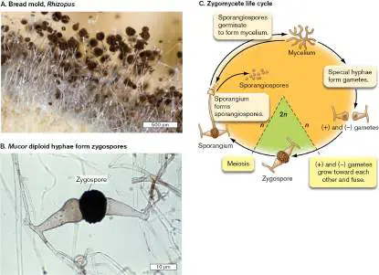
form a zygospore. The zygospore undergoes meiosis and generates the sporangium, a
haploid structure that releases sporangiospores.
Thought Question
20.4 What are the advantages and limitations of motile gametes, as compared to
nonmotile spores?
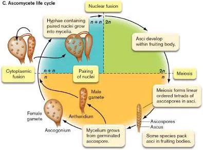
Ascomycota: mycelia with paired nuclei. The ascomycete fungi are famous in the
history of science, as well as in the culinary arts (Fig. 20.13 ). The bread mold
Neurospora was used by George Beadle and Edward Tatum in the 1940s to formulate
the one gene–one protein theory. In Neurospora, meiosis produces pods (asci) of
ascospores aligned in rows that reflect the ordered tetrads of meiotic division (Fig.
20.13A ). The tetrad patterns were used by geneticists to demonstrate the segregation
and independent assortment of chromosomes. In other species, by contrast, the asci are
packed in large mushroom-like fruiting bodies known as morels (Morchella hortensis;
Fig. 20.13B ) and truffles (Tuber aestivum). The ascospores of such fruiting bodies
are spread by animals attracted by their delicious flavor. Human collectors traditionally
use muzzled pigs to detect and unearth the famous underground truffles.
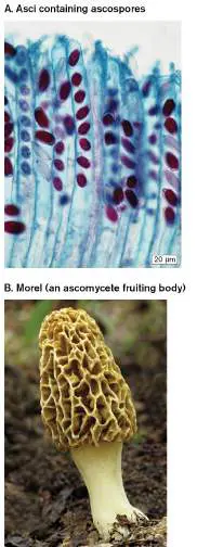
FIGURE 20.13 ■ Ascomycetes produce large fruiting bodies. A.
Ascomycete asci containing ascospores (stained red). B. The culinary delicacies
known as morels are fruiting bodies of the species Morchella hortensis. The dark
pits of the morel are lined with asci. C. The life cycle of an ascomycete alternates
between the diploid and haploid forms. The diploid mycelium produces asci, within
which the haploid ascospores are formed.
ED RESCHKE/PETER ARNOLD/GETTY IMAGES
ED RESCHKE/PETER ARNOLD/GETTY IMAGES
The ascomycete life cycle (Fig. 20.13C ) includes a phase in which each cell
possesses a pair of separate nuclei, one from each parent (chromosome number is
designated n + n). The “dikaryotic” (paired-nuclei) phase is generated by haploid
mycelia in which male and female reproductive structures fuse, followed by migration of
all the male nuclei into the female structure. The paired nuclei then undergo several
rounds of mitotic division while migrating into the growing mycelium. In the mycelial
tips, the paired nuclei finally fuse (becoming 2 n), and the mycelial tips develop into
asci. Each ascus then undergoes meiosis in which the haploid products segregate in the
same order that the meiotic chromosomes separated.
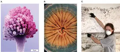
Some ascomycetes, such as Aspergillus and Penicillium species, form small asexual
fruiting bodies called conidiophores for airborne spore dispersal (Fig. 20.14A ).
Penicillium is known for producing penicillin, the first antibiotic in widespread use; forms
of penicillin are still used today (discussed in Chapter 1). Aspergillus (Fig. 20.14A
and B ) is a growing medical problem as an opportunistic pathogen of
immunocompromised patients. Aspergillus can produce toxins (called mycotoxins) such
as aflatoxin. Aflatoxin poisoning commonly affects livestock and, in some cases,
agricultural workers; the toxin causes liver damage, immunosuppression, and cancer.
FIGURE 20.14 ■ Ascomycete molds. A. Aspergillus forms a microscopic
asexual fruiting structure called a conidiophore, containing spores in its spherical
tip. B. Colony of Aspergillus nidulans on an agar plate. C. Black mold (such as
Stachybotrys) grows above the flood line on a kitchen wall. An undergraduate
volunteer points out the presence of mold in New Orleans, 6 months after flooding
caused by Hurricane Katrina.
DR. DAVID M. PHILLIPS/VISUALS UNLIMITED
SCIENCE PHOTO LIBRARY/SCIENCE SOURCE
JOAN SLONCZEWSKI
Conidiophore-forming ascomycetes such as Aspergillus and Stachybotrys are the
major forms of mold associated with dampness in human dwellings; for example, they
caused massive damage to homes flooded in the wake of Hurricane Katrina in 2005 (
Fig. 20.14C ). The flooding of homes full of drywall made ideal conditions for the
growth of mold, which commonly consists of airborne ascomycete mycelia. Mold grew
not only on materials submerged, but also on the surface above exposed to water-
saturated air, up to 3 feet above the flood line (the highest level submerged).
Unfortunately, most homeowner insurance policies covered damage only “up to the
flood line.”
Many ascomycetes are pathogens of animals or plants. For example, Microsporum
and Trichophyton species cause ringworm skin infection, whereas Magnaporthe oryzae
causes rice blast, the most serious disease of cultivated rice. Other species, however,
are beneficial symbionts of plants, including crop plants such as beans, cucumbers, and
cotton. Trichoderma species grow on the roots or, in some cases, within the vascular
tissue of the plant. The fungi share nutrients with the plant, and they induce plant
defenses against pathogens. Trichoderma even has a commercial use in cloth
processing; the fungus is used to make “stonewashed jeans,” as its cellulase enzymes
partly digest the cotton.
Thought Question
20.5 Compare the life cycle of an ascomycete (Fig. 20.13C ) with that of a
chytridiomycete (Fig. 20.11C ). How are they similar, and how do they differ?
Basidiomycota: cells with paired nuclei form mushrooms. The basidiomycetes
form large, intricate fruiting bodies known as “true” mushrooms (Fig. 20.15 ).
Mushrooms produce some of the world’s deadliest poisons, such as alpha-amanitin,
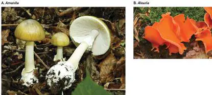
which inhibits RNA polymerase II. Alpha-amanitin is produced by the amanita, or
“destroying angel” (Fig. 20.15A ), a taste of which is usually fatal. (The amanita’s
own RNA polymerase is insensitive to the toxin.)
FIGURE 20.15 ■ Mushrooms and other complex fruiting bodies. A. The
basidiomycete mushroom Amanita phalloides makes one of the most dangerous
toxins known: alpha-amanitin, an inhibitor of RNA polymerase II. B. The
ascomycete Aleuria aurantia, “orange fungus.”
EL_CIGARRITO/SHUTTERSTOCK
ARCO IMAGES GMBH/ALAMY STOCK PHOTO
Other mushroom species include some of the world’s most prized culinary delights,
such as the portobello. Many grow in soil, while others, such as Piptoporus, grow on
tree bark. Some mushrooms have evolved elaborate insect-attracting structures and
odors, such as the “starfish stinkhorn,” with its ring of bright red horns.
The mushroom itself is only the fruiting body of the basidiomycete. The
basidiomycete life cycle involves transitions among n, n + n, and 2 n (Fig. 20.16A )
similar to those of ascomycetes (see Fig. 20.13C ). In the basidiomycete, however, the
fruiting body consists largely of cells with paired nuclei (n + n). A few of the paired
nuclei fuse to form diploid cells (2 n) called basidia (singular, basidium), which line the
gills of the mushroom. The basidia undergo meiosis to form haploid basidiospores (n).
Some types of basidia can release basidiospores under pressure, whereas other
basidiospores are dispersed by wind. Some fungi that resemble mushrooms, such as
Aleuria, are actually classified as ascomycetes (Fig. 20.15B ).
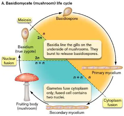
FIGURE 20.16 ■ Mushroom life cycle. A. Haploid basidiospores generate
primary mycelium underground, where they form gametes. Gametes of opposite
mating types fuse their cytoplasm only, forming secondary mycelium. The parental
nuclei remain separate throughout many generations of mitosis during development
of the fruiting body (mushroom). As the mushroom matures, the basidia undergo
nuclear fusion and meiosis, forming progeny basidiospores. B. The underground
secondary mycelia of some mushrooms form mycorrhizae with tree roots.
Mycorrhizae enhance and extend the absorptive power of the tree roots, while
obtaining plant sugars for the fungus.
The basidiospores germinate to form underground mycelium. This haploid “primary
mycelium” generates gametes that ultimately fuse to form n + n “secondary mycelium.”
The primary and secondary mycelia may radiate underground, unseen, until their tips
generate mushrooms aboveground, at points approximately equidistant from the origin.
The result is a mysterious “fairy ring” of mushrooms (Fig. 20.3A). In a forest, these
invisible underground hyphae of basidiomycetes contribute filaments of mycorrhizae
(singular, mycorrhiza). Mycorrhizae are filamentous fungi that gain sugars from trees
while extending the tree root systems (Fig. 20.16B ). The mycorrhizae formed by
mushrooms are called “ectomycorrhizae” because their hyphae coat the plant roots but
do not penetrate plant cells.
Glomeromycota form arbuscular mycorrhizae that penetrate plant cells. A
remarkable group of fungi is the Glomeromycota, class Glomeromycetes, all of which
are obligate mutualists of plants. These fungi, such as Glomus species, form extensive
networks of filamentous connections with plant roots similar to the mycorrhizae formed
by basidiomycete. But unlike the basidiomycete mycorrhizae, the mycorrhizae formed
by glomeromycota are arbuscular mycorrhizae, also called endomycorrhizae, in which
the fungal hyphae actually penetrate plant cells in a most intimate symbiosis (Fig.
20.17 ). Mycorrhizae expand the roots’ absorptive capacity, while obtaining plant
sugars for the fungus. More than 90% of all land plants, including trees, depend on
these fungal interconnections, which share nutrients among many different plants and
even different species, as well as among fungi (discussed in Chapter 21). The health of
entire forests requires a “world wood web” of fungi.
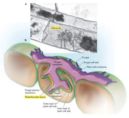
FIGURE 20.17 ■ Arbuscular mycorrhiza. A. Glomeromycota fungi invade corn
root cells as part of a mutualistic symbiosis to exchange nutrients. B. The fungal
hypha grows between the plant cells, and then into a plant cell to form an
arbuscule. The arbuscule expands surface area for exchange while maintaining the
plant cell membrane intact.
Source: Part B modified from Martin Parniske. 2008. Nat. Rev. Microbiol. 6 :763.
USDA
In arbuscular mycorrhizae, a fungal hypha first grows between plant cells without
breaching the plant cell wall (Fig. 20.17B ). Next, the hypha branches into the plant
cell, growing through a breach in the outer later of cell wall. The hypha invaginates the
inner layer of cell wall without penetrating the cell membrane. The plant cell membrane
invaginates to accommodate the branch, while maintaining a “periarbuscular space”
between the plant cell membrane and the fungal plasma membrane. This highly
regulated invaginating branch is called an “arbuscule”—hence the term “arbuscular
mycorrhiza.” Arbuscule formation is regulated by plant hormones called strigolactones.
The arbuscule expands the surface area to exchange sugars from the plant for
ammonium and phosphate from the fungus.
Emerging Fungal Pathogens
The dominant role of fungi in our biosphere is positive—as decomposers, recyclers, and
symbiotic partners within lichens and mycorrhizae (discussed further in Chapter 21).
But some fungi are important pathogens, such as Histoplasma capsulatum, an
ascomycete fungus that infects healthy people who inhale contaminated dust, causing a
deadly pneumonia. And as human demographics shift and climate change increases, a
growing number of human, animal, and plant pathogens emerge (Table 20.2 ). For
immunocompromised patients, especially the elderly confined to hospitals, a growing
threat is Aspergillus species, which can colonize the lungs and other tissues. In 2012,
contaminated steroid injections led to an outbreak of infections by Exserohilum
rostratum and other previously rare opportunists. Other fungal pathogens cause
massive mortality of animals and plants.
Emerging Fungal and Microsporidian TABLE 20.2 Pathogens
Species Phylum Host Disease
Aspergillus Ascomycota Humans Aspergillosis of lung,
fumigatus (immunocompromis and elsewhere in
ed) the body
Batrachochytrium Chytridiomycota Amphibians (frogs and Chytridiomycosis
dendrobatidis toads)
Cryptococcus Basidiomycota Humans Meningitis and
neoformans (immunocompromis meningoencephali
ed) tis
Emerging Fungal and Microsporidian TABLE 20.2 Pathogens
Species Phylum Host Disease
Encephalitozoon Microsporidia Humans with AIDS Microsporidiosis
intestinalis (intestinal)
Exserohilum Ascomycota Humans Wound and skin
rostratum infections;
contaminated
injections
Fusarium solani Ascomycota Sea turtles Hatch failure
(loggerheads)
Pseudogymnoascus Ascomycota Brown bats White nose disease
destructans
Histoplasma Ascomycota Humans, dogs, cats Histoplasmosis
capsulatum (lung)
Magnaporthe Ascomycota Rice Rice blast disease
oryzae
Nosema species Microsporidia Honeybees Colony collapse
disorder
Pneumocystis Ascomycota Humans Pneumocystis
jirovecii (immunocompromis pneumonia
ed)
Puccinia graminis Basidiomycota Wheat Wheat stem rust
Stachybotrys Ascomycota Humans Black mold disease;
chartarum respiratory
damage
Several parasitic organisms originally classified as protozoa because of their
superficial appearance have since been shown to be fungi or fungus-related on the basis
of their genome sequence and biochemistry. The reclassification has important
consequences for research, taxonomy, and therapy. An example is the ascomycete
Pneumocystis jirovecii. The organism was first described in 1909, when it was thought
to be a life stage of a trypanosomatid causing Chagas’ disease (discussed in Section
20.6). When the organism was recognized as a distinct species of protist infecting
animals, it was named Pneumocystis carinii. In the 1970s, this strain of Pneumocystis
was renamed P. jirovecii for causing pneumonia in immunocompromised humans. In the
1980s, the rise of AIDS led to a sudden increase in infections. Sequencing the
organism’s genome revealed it to be an ascomycete fungus. As a result, the organism’s
developmental forms and biochemistry were reevaluated, and medical research was
redirected to culture and treat the organism on the basis of fungal physiology.
A major clade of parasites closely related to fungi is Microsporidia. Microsporidia
have relatively small genomes; their mitochondria have lost their DNA and no longer
generate ATP for the cell. Microsporidia form spores as small as a few micrometers in
size, which can infect animal cells. The microsporidian spore extrudes a specialized
invasion complex, called the polar tube, that penetrates the host cell, typically a
macrophage. In humans, microsporidians are opportunistic pathogens, such as the
intestinal parasite Encephalitozoon intestinalis, emerging with the rise of AIDS and the
growth of elderly and immunocompromised populations.
Other taxa originally assigned as fungi because of superficial appearance have been
reclassified within protist clades on the basis of cell biology and genome sequences. The
Oomycetes (formerly called Oomycota, or “water molds”) were originally classified as
fungi because of their fungus-like filaments, which infect plants and animals. Based on
genome sequences, Oomycetes are now classified as Stramenopiles (supergroup SAR).
The oomycete Phytophthora infestans devastated Irish potato crops in the 1840s,
causing the Great Irish Famine, in which a million people died. Today P. infestans still
causes outbreaks of “potato blight,” a problem for agriculture worldwide. A related
species, Phytophthora ramosum, causes “sudden oak death,” a disease killing tens of
thousands of oaks and other trees in the western United States.
To Summarize
Fungi form hyphae with cell walls of chitin. Hyphae absorb nutrients from
decaying organisms or from infected hosts. Some fungi remain unicellular; these
are called yeasts or mitosporic fungi.
Chytridiomycete fungi have motile zoospores. Motile reproductive forms
are a trait shared with animals. Flagellar motility has been lost by other fungi
through reductive evolution.
Zygomycete fungi form haploid mycelia. Hyphal tips differentiate into
gametes and grow toward each other to undergo sexual reproduction.
Ascomycete fungal mycelia form paired nuclei. Within some of these
dikaryotic cells, the paired nuclei fuse, followed by meiosis and development of
ascospores. Some ascomycetes form asexual spores via structures called
conidiophores.
Basidiomycete fungi form mushrooms. Cells with paired nuclei (secondary
mycelium) form large fruiting bodies called mushrooms. The paired nuclei fuse to
form the diploid basidium, which generates haploid basidiospores. The
basidiospores develop underground hyphae or mycorrhizae that interconnect
plant roots.
Glomeromycota form arbuscular mycorrhizae. These fungi form intimate
mutualistic networks of connections with the roots of trees and other plants,
exchanging minerals for plant sugars.
Emerging fungal pathogens threaten humans, plants, and animals.
Glossary
hypha pl. hyphae
The threadlike filament that forms the mycelium of a fungus.
mycelium pl. mycelia
A single mass of fungal hyphae that projects into the air (aerial mycelium) or into
the growth substrate (surface mycelium).
yeast
A unicellular fungus.
budding
A form of reproduction in which mitosis of the mother cell generates daughter cells
of unequal size.
mitosis
The orderly replication and segregation of eukaryotic chromosomes, usually prior to
cell division.
alternation of generations
A life cycle that alternates between populations of haploid cells and diploid cells,
which undergo meiosis and fertilization.
ascus pl. asci
A spore-containing pod produced by ascomycete fungi.
mitosporic fungus
Also called imperfect fungus. A species of fungus that generates spores by mitosis
and lacks a known sexual cycle.
zygomycete
A member of the eukaryotic group Zygomycota—fungi forming nonmotile haploid
gametes that grow toward each other, fusing to form the zygospore.
sporangium pl. sporangia
A fungal organ that releases nonmotile spores.
zygospore
In zygomycetes, the diploid structure formed by the fusion of two gamete-bearing
hyphae.
sporangiospore
A haploid spore of a fungus that can germinate to form a haploid mycelium.
ascomycete
A member of the eukaryotic group Ascomycota—fungi whose mycelia form paired
nuclei. Haploid ascospores are produced in pods called asci.
ascospore
The spore produced by an ascomycete fungus.
basidiomycete
A member of the eukaryotic group Basidiomycota—fungi that form mushrooms.
basidiospore
A haploid spore formed by a basidiomycete through meiosis of a basidium, a
reproductive cell of a mushroom.
mycorrhizae sing. mycorrhiza
Fungi involved in an intimate mutualism with plant roots, in which nutrients are
exchanged.
arbuscular mycorrhizae
Also called vesicular-arbuscular mycorrhizae or endomycorrhizae. Mutualistic
associations between plant roots and certain fungi, involving hyphal penetration of
plant root cells.
Oomycetes
Formerly called water molds. A member of the eukaryotic group Oomycetes—
heterokont protists whose life cycle resembles that of fungi; formerly classified as
fungi (Oomycota).
Fig. 20.3A
FIGURE 20.3 ■ Traditional views of fungi and protozoa (protists). A.
Basidiomycete mushrooms growing in a “fairy ring.” B. A nineteenth-century
depiction of various protozoa, by Rudolf Leuckart.
NASTASIC/GETTY IMAGES
20.3 Amoebozoa: Amebas and Slime Moldsnot assigned
The ameba (alternative spelling “amoeba”) is familiar to most of us as an apparently amorphous form of microscopic life, capable of engulfing and consuming prey in a dramatic fashion. Amebas are a polyphyletic group; that is, the group lacks a common ancestor and includes members that branch from distantly related clades. The taxonomy of amebas and slime molds remains problematic, with diverse views as to the number of clades, their relatedness, and their degree of divergence. Here we discuss the amebas of the Amoebozoa clade (Fig. 20.4). This group includes solitary amebas as well as “social” amebas called slime molds that aggregate to form a multicellular fruiting body.
An ameba’s shape is exceptionally variable, but the pseudopods, or “false feet” (Fig. 20.18), that it extends are complex structures that undertake highly controlled movements. The “classic” amebas of the Amoebozoa are free-living predators in soil or water, engulfing prey by phagocytosis. They range in size up to 5 mm, large enough to phagocytose bacteria, algae, ciliates, smaller amebas, and even invertebrates such as rotifers. A few are dangerous parasites of humans or animals. Furthermore, free-living amebas can harbor bacterial pathogens such as Legionella pneumophila, which contaminates water supplies and air ducts. The bacteria cause legionellosis, an often fatal form of pneumonia. The host ameba enables the pathogen’s persistence and transmission to human hosts.
FIGURE 20.18 ■ Amoeba proteus moves by extending its pseudopods.
M. I. WALKER/SCIENCE SOURCE
Free-living amebas such as Acanthamoeba species are common predators in the soil microbial community. They cause problems when they contaminate contact lens cleaning solutions, causing keratitis (infection of the cornea). Wearers of contact lenses have an increased risk of Acanthamoeba keratitis.
Pseudopod Motility Thought Question
20.6 What cellular interactions can happen when an ameba phagocytoses algae?
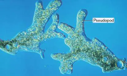
Species from diverse clades form ameba-like cells with pseudopods. The Amoebozoa persist as an ameba throughout all or most of the life cycle. Other protists can convert to flagellated forms, particularly when the habitat fills with water—a low-viscosity condition favoring flagellar motility. For example, Naegleria fowleri, the “brain-eating ameba,” is a parasite of the Discoba group of parasitic protists ( Section 20.6). A pond organism that causes amebic meningoencephalitis, N. fowleri exists as a flagellate and as an ameboid form with pseudopods. Other species such as dinoflagellates never become fully ameboid, but they can extend a pseudopod to engulf prey.
Different kinds of amebas have different kinds of pseudopods. Many of the Amoebozoa have lobe-shaped pseudopods (Fig. 20.18 ). Lobe-shaped pseudopods have the most variable shape. Another form is the sheetlike pseudopod, or lamellar pseudopod, used by some Amoebozoa. Lamellipodia also evolved independently in the distantly related dinoflagellates (Section 20.5). Similar lamellar pseudopods are generated by human white blood cells such as leukocytes. Finally, needlelike pseudopods, or filopodia, are thin extensions reinforced by parallel actin filaments. These are typical of Rhizaria amebas, although some Rhizaria instead make long, thin pseudopods supported by microtubules. The most famous protists with microtubule-supported pseudopods also have mineralized supporting structures, such as Foraminifera (spiral shells) and Radiolaria (radial-form “skeleton”).
The extension of lobe-shaped and lamellar pseudopods has been studied closely for its relevance to human white blood cells (for more on white blood cells as host defenses, see Chapter 23). The mechanism of pseudopod motility involves a sol-gel transition between cortical cytoplasm (just beneath the cell surface) and the cytoplasm of the deeper interior (Fig. 20.19). The tip of a pseudopod contains a gel of polymerized actin-myosin beneath its cell membrane. From the center of the ameba, liquid cytoplasm (sol) containing actin subunits streams forward along microtubular “tracks,” powered by ATP hydrolysis. The actin subunits stream into the pseudopod, where they polymerize, forming a gel. The gel region grows, pushing the membrane forward and extending the pseudopod. As the gel is pushed backward, it resolubilizes to continue the cycle.
FIGURE 20.19 ■ Pseudopod motility . A pseudopod extends by flow of liquid cytoplasm (sol state) followed by actin polymerization (gel state). As actin polymerizes, the cell rotates down toward the substrate like a tank tread.
Amebas can have one nucleus or multiple nuclei, and some species are polyploid (possess multiple copies of the genome). They are usually haploid and reproduce asexually by nuclear mitosis, without dissolution of the nuclear membrane, followed by fission of the cytoplasm. Some species do have developmental alternatives, such as cyst formation, gamete fusion and meiosis, and even growth of flagella in a favorable habitat.
Thought Question
20.7 What kind of habitat would favor a flagellated ameba?
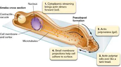
Ameba genetics is poorly understood, but one ameba genome that has been sequenced is that of the intestinal parasite Entamoeba histolytica. The E. histolytica sequence contains 27 Mb of DNA in 38 chromosomes; some of these are linear, whereas others are circular. Closely related strains show considerable variation in organization, suggesting that ameba genomes undergo extensive rearrangement.
Slime Molds
Some amebas conduct a life cycle in which thousands of individuals (all members of one species) aggregate into a complex, differentiated fruiting body (Fig. 20.20A). Such an organism is called a cellular slime mold. A cellular slime mold forms from ameboid cells that aggregate into a multicellular “slug.” Slime molds, as the name implies, were originally classified with fungi because their fruiting bodies superficially resemble fungal reproductive forms. FIGURE 20.20 ■ A cellular slime mold: Dictyostelium discoideum. A. Fruiting bodies of D. discoideum (composite SEM). B. D. discoideum aggregation of cells, mediated by waves of cAMP signal. Green fluorescence indicates cAMP binding a cAMP-dependent fluorophore, Flamindo2. C. Life cycle of D. discoideum.
Source: Inset from Hidenori Hashimura et al. 2019. Commun. Biol. 2 :34.
DAVID SCHARF/SCIENCE SOURCE
H. HASHIMURA ET AL. 2019. COMMUN BIOL. 2 :34
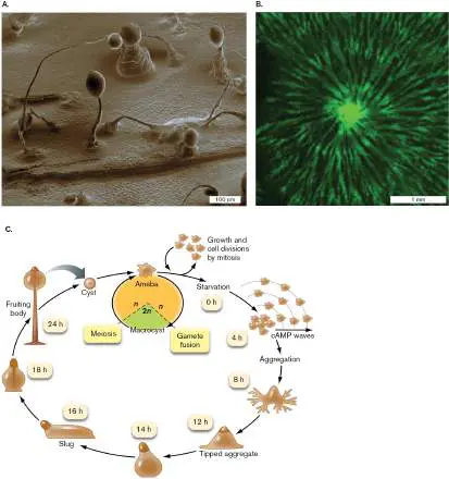
A well-studied example of a cellular slime mold is Dictyostelium discoideum, historically an important model system for multicellular development (Fig. 20.20). D. discoideum amebas are relatively small, about 10 μm, but large enough to consume bacteria. They can be cocultured on a plate with Escherichia coli. As the haploid amebas consume bacteria, they divide asexually until their food runs out. At this point, a few amebas begin to emit the aggregation signaling molecule cyclic AMP (cAMP). An ameba emitting cyclic AMP attracts other amebas nearby, which move toward the center and begin emitting cyclic AMP as well. Successive waves of cyclic AMP continue to attract thousands of amebas aggregating at the center, where they pile on top of each other.
The aggregating cells form a multicellular slug that extends as long as 1 mm. The slug then migrates, attracted by light and warmth, to find an appropriate place to form a fruiting body and disperse its spores. At last, the slug differentiates into a fruiting body, a spherical sporangium supported on a stalk of largely empty cells that emerges from a basal disk. The sporangium then releases spores (also called cysts), which are dispersed on air currents and can remain viable for several years. When a spore detects chemical signals from bacteria, it germinates as an ameba to feed on them. Note that the entire reproductive cycle just described is asexual; the amebas and their differentiated structures remain haploid throughout. D. discoideum amebas do have a sexual alternative (illustrated in Fig. 20.20C ), in which cells of opposite mating type can fuse to form a diploid zygote and then undergo meiosis, restoring the haploid state of amebas.
A different kind of slime mold is the plasmodial slime mold, in which an ameba undergoes mitosis without cell division, forming a multinucleate single cell. A plasmodial slime mold such as Physarum polycephalum develops from a single diploid ameba. As the ameba grows, its nuclei multiply, forming a plasmodium (plural, plasmodia ), a giant multinucleate cell that can spread over an area of many square centimeters. Out of the plasmodium arise fruiting bodies whose sporangia undergo meiosis, producing haploid spores. The spores later germinate as haploid amebas (or flagellates, for some species). Under appropriate conditions, two amebas or flagellates fertilize each other to form a diploid ameba that can develop again into a plasmodium. A large plasmodium can occasionally be seen as a yellow mass of slime spreading over decaying wood.
Note: Distinguish the term “plasmodium” (a large multinucleate
cell) from the genus Plasmodium (an apicomplexan parasite, such as Plasmodium falciparum, which causes malaria).
Filamentous and Shelled Amebas
The Rhizaria form needlelike pseudopods. Despite the term “filamentous amebas,” the Rhizaria form a clade distant from the classic amebas, within supergroup SAR (see Section 20.5). Some Rhizaria are encased by mineral shells called tests. A major group is the radiolarians, whose skeletons are made of silica perforated with numerous holes through which pseudopods appear to radiate in all directions (Fig. 20.21A). Radiolarians grow in marine and freshwater habitats. Many different kinds of radiolarians exist today, and many can be recognized in fossil rock.
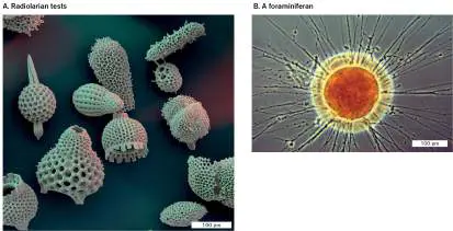
FIGURE 20.21 ■ Filamentous and shelled amebas. A. Shells (tests) of radiolarians (stereoscope). B. A live foraminiferan, Allogromia (dark-field).
EYE OF SCIENCE/SCIENCE SOURCE
GREG ANTIPA/SCIENCE SOURCE
A second group of shelled amebas is the foraminiferans (Fig. 20.21B ). The foraminiferans, or forams, generate shells of calcium carbonate as chambers laid down in helical succession. Their pseudopods all extend from one opening in the most recent chamber. The shells of dead forams make important contributions to marine sediment and ancient rock formations. Forams are used in geological surveys as indicators of petroleum deposits.
To Summarize
Amebas move using pseudopods. In different species, pseudopods are lobe-shaped, lamellar, or filamentous (filopodia).
Cytoplasmic streaming through cycles of actin polymerization and depolymerization drives the extension and retraction of pseudopods.
Slime molds have a life history stage in which a fruiting body produces spores. In cellular slime molds, amebas aggregate to form a slug. In plasmodial slime molds, a single ameba develops into a giant multinucleate cell.
Radiolarians have silica skeletons and form filamentous pseudopods.
Foraminiferans have calcium carbonate shells with helical arrangement of chambers. The most recent chamber opens to extend filamentous pseudopods.
Amebas such as Acanthamoeba, Entamoeba, and Naegleria are parasites of humans. Many other amebas of diverse groups are free-living.
Glossary
phagocytosis A form of endocytosis in which a large extracellular particle is brought into the cell.
cellular slime mold A slime mold in which the individual bacterial cells retain their own cell membranes; not a fungus.
plasmodial slime mold A slime mold in which a fertilized zygote undergoes multiple nuclear divisions, generating a multinucleate single cell (plasmodium).
plasmodium pl. plasmodia The giant, multinucleate cell formed by a plasmodial slime mold.
radiolarian A member of the eukaryotic group Radiolaria—amebas with a silicate shell penetrated by filamentous pseudopods. foraminiferan or foram An ameba with a calcium carbonate shell and a helical arrangement of chambers.
Fig. 20.4 FIGURE 20.4 ■ Eukaryotic phylogeny. A phylogenetic tree of major clades (supergroups) of eukaryotes based on DNA sequence data. Dotted lines denote uncertain lineage. Green asterisks denote secondary algae whose ancestor engulfed a primary alga with chloroplast.
Sources: Modified from Sandra L. Baldauf. 2003. Science 300 :1703; and Fabien Burki et al. 2020. Trends Ecol. Evol. 35 :43.
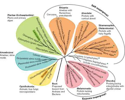
20.4 Algaenot assigned
Algae are eukaryotic microbes that contain a chloroplast. They fix CO 2 in all ecosystems, most crucially freshwater and marine habitats. In freshwater and marine ecology, the algae, together with photosynthetic bacteria, are known as phytoplankton (see Chapter 21 ).
The primary algae (supergroup Plantae or Archaeplastida) are products of a single ancestral endosymbiosis that also gave rise to land plants. The biochemistry and cell structures of green algae and land plants are similar; thus, the alga Chlorella was the model organism of choice for pioneers of CO 2 fixation, including Martin Kamen, Melvin Calvin, and others (discussed in Chapter 15).
Other photosynthetic eukaryotes, or secondary endosymbiotic algae, arose from protists that engulfed a primary or secondary alga. In the SAR supergroup, distinct endosymbiotic events led to dinoflagellates (in the Alveolata) and to kelps and diatoms (in the Stramenopiles). Secondary algae often show “mixotrophic” nutrition, involving both phototrophy and heterotrophy. For example, dinoflagellate “algae” are voracious predators of smaller protists. The stramenopile algae (diatoms and kelps) and the coccolithophores are covered in this section, after the primary algae. Dinoflagellates are covered under alveolates (Section 20.5).
Primary Algae
The primary endosymbiotic algae include two major clades: Chlorophyta, or green algae; and Rhodophyta, or red algae—although not all members of each group appear green or red, respectively. Rhodophyta that appear red have a secondary pigment called phycoerythrin, in addition to green chlorophyll.
Green algae (Chlorophyta). Many green algae are unicellular. An important model system for genetics and phototaxis is Chlamydomonas reinhardtii, a unicellular chlorophyte common in freshwater systems as well as Antarctic pools. The genetics of cell cycle regulation in C. reinhardtii provides clues to the formation of human tumors.
C. reinhardtii has a symmetrical pair of flagella—a common pattern for green algae and their gametes (Fig. 20.22A). The alga swims forward by bending its flagella back toward the cell, like a breaststroke. Chlamydomonas cells are mostly haploid, reproducing by asexual cell division (Fig. 20.22B ). For sexual reproduction, opposite mating types fuse to form a zygote, which loses flagella and grows a spiny protective coat. The zygote undergoes meiosis to regenerate haploid cells.
FIGURE 20.22 ■ A single-celled green alga: Chlamydomonas reinhardtii. A. Chlamydomonas has a green chloroplast and grows as a photoautotroph. A symmetrical pair of flagella pulls the cell forward. B. Alternation of generations. Chlamydomonas reproduces asexually as haploid cells.
Alternatively, the alga generates gametes that fuse into a zygote that immediately undergoes meiosis to regenerate haploid cells.
J. L. CARSON, PH.D/SCIENCE SOURCE
The cell ultrastructure of Chlamydomonas is typical of algal cells ( Fig. 20.23). The nucleus is cupped by a single chloroplast, which is
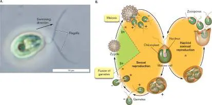
surrounded by a double membrane. The double membrane indicates primary algae; the inner membrane derives from the ancestral bacterium, and the outer membrane derives from the engulfing host. Within the chloroplast is a pyrenoid, an organelle that in some species concentrates bicarbonate (HCO −) and converts it to CO
3 2
for fixation. The pyrenoid is surrounded by one or more starch bodies, which are used for energy storage. The starch is broken down to sugars as needed, followed by glycolysis and respiration in the mitochondria. Osmolarity is maintained by the contractile vacuole. The Chlamydomonas cell is encased in a cell wall composed predominantly of glycoprotein. Other green algae have cellulose cell walls similar to those of plants.
FIGURE 20.23 ■ Cell structure of Chlamydomonas reinhardtii. A . The cell membrane is surrounded by a cell wall of cellulose and glycoproteins. The single chloroplast fills much of the cell and wraps around the nucleus. Within the chloroplast lies a pyrenoid, a structure for concentrating bicarbonate ion for conversion to CO 2. The pyrenoid is surrounded by starch bodies that store high-energy compounds. A contractile vacuole maintains constant osmotic pressure. B. Electron micrograph of C. reinhardtii shows the nucleus, chloroplast, pyrenoid, and other organelles.
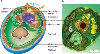
AMI IMAGES/SCIENCE SOURCE
While C. reinhardtii is unicellular in nature, some marine and freshwater algae that resemble Chlamydomonas grow naturally in intricate multicellular colonies. Colonial algae such as Volvox (Fig. 20.24B ) generate geodesic spheres of biflagellate cells. Their flagella point outward from the colony, propelling it forward and drawing nutrients across its surface. Each cell of Volvox connects by cytoplasmic bridges to five or six of its neighbors. The colony reproduces by generating daughter colonies within the sphere, which grow until the outer sphere falls apart, liberating the daughters.
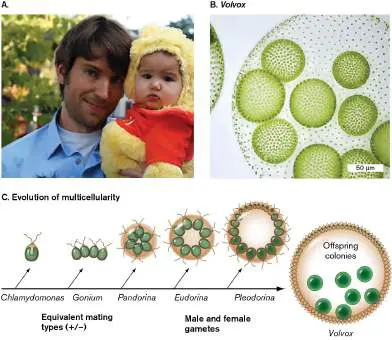
FIGURE 20.24 ■ Single-celled algae can evolve multicellularity . A. William Ratcliff, whose lab studies origins of multicellularity, with his own multicellular offspring. B. Volvox algae form a spherical colony of cells (1–3 mm) that generates offspring colonies within. C . Different types of algae suggest a model for the evolution of multicellularity from a unicellular ancestor (like Chlamydomonas) to a multicellular colony with female and male gametes (Volvox). D, E. Chlamydomonas reinhardtii after evolution for 750 generations, without predation and with predation. Source: Parts D and E from Matthew Herron et al. 2019. Sci. Rep. 9 :2328.
COURTESY OF WILLIAM RATCLIFF
FRANK FOX/SCIENCE SOURCE
M. D. HERRON ET AL. 2019. SCI REP. 9 :2328
M. D. HERRON ET AL. 2019. SCI REP. 9 :2328
Could single-celled algae evolve multicellularity? An experiment shows that, under selection pressure, C. reinhardtii can quickly evolve into a multicellular form. William Ratcliff at the Georgia Institute of Technology (Fig. 20.24A) and Michael Travisano at the University of Minnesota showed that C. reinhardtii could undergo selection by repeated subculturing in a standing tube. In each culture, a few cells would clump at the bottom, and the clumps were selectively cultured further. Eventually, a strain was isolated that grew regularly in connected cell clusters that alternated with dispersal. Ratcliff further showed that over many generations, predation by paramecia could select for C. reinhardtii clones that grow only as clumps. Compare the
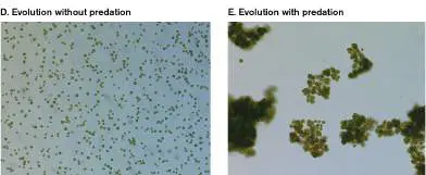
control population (Fig. 20.24D ) with a strain that evolved in the presence of predatory Paramecium (Fig. 20.24E ).
A survey of algal diversity from Chlamydomonas through Volvox suggests a model for the progression of evolving multicellularity ( Fig. 20.24C ). First, cells might have evolved to grow in small, ordered structures, as is seen for Gonium and Pandorina species. The structures then might have evolved into hollow spheres of cells with some differentiation, as seen in Eudorina. Male and female gametes then evolved (Pleodorina), and ultimately colonies that generate colonial offspring (such as Volvox).
Other species of algae grow as multicellular filaments. An example is Spirogyra, a common pond dweller known for its spiral chloroplasts (Fig. 20.25A). As with Chlamydomonas, the haploid form predominates; but unlike the unicellular alga, Spirogyra forms neither flagellated gametes nor zoospores. Instead, its sexual reproduction requires alignment of two filaments of opposite mating type (Fig. 20.25B ). Cells conjugate (form cytoplasmic bridges) between the two filaments. The “male” gametes are those whose cytoplasm inserts through the conjugation bridge to join that of the “female” gamete. As the gametes fuse, a row of empty cell walls is left behind (Fig. 20.25C ). The zygote eventually hatches and germinates a new chain of cells.
FIGURE 20.25 ■ Filaments with spiral chloroplasts: Spirogyra. A. Spirogyra species grow in long, multicellular filaments, typically 25 μm wide and several centimeters long. Each cell contains one or more chloroplasts that spiral around the
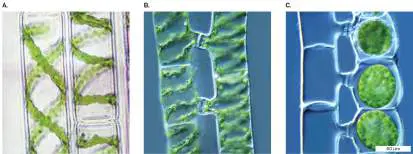
cytoplasm. B . Sexual reproduction involves conjugation between cells of two mating types. The cytoplasm from each male cell exits its cell wall and enters the female cell. C. Gamete fusion is complete, generating zygotic spores.
BIOPHOTO ASSOCIATES/SCIENCE SOURCE
M. I. WALKER/SCIENCE SOURCE
M. I. WALKER/SCIENCE SOURCE
Some marine algae grow in extensive, undulating sheets. An example familiar to beach bathers is the “sea lettuce” Ulva (Fig. 20.26A). Sheets of Ulva can extend over many square meters, although they are only two cells thick (see Fig. 20.26A, inset). Ulva and other algae produce diverse molecules with potentially useful pharmaceutical properties as antimicrobial and anti-inflammatory agents.
FIGURE 20.26 ■ Multicellular algae: Ulva. A. Ulva species generate large, undulating sheets of cells in double layers (inset). B. Ulva undergoes symmetrical alternation of generations. The haploid and diploid forms appear very similar.
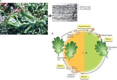
Source: Part B modified from Christine Bobin-Dubigeon et al. 1997. J. Sci. Food Agric. 75 :341–351.
BIOPHOTO ASSOCIATES/SCIENCE SOURCE; INSET: C. BOBIN-DUBIGEON ET AL. 1997.
J. SCI. FOOD AGRIC. 75 :341–351.
The Ulva life cycle shows classic alternation of generations between haploid and diploid forms (Fig. 20.26B ). Haploid sheets of cells (the gametophyte) produce symmetrically biflagellate gametes, similar to unicellular Chlamydomonas. But when Ulva gametes fuse, the zygote grows into an immense diploid sheet of cells. This sporophyte (diploid multicellular body) appears similar in form to the gametophyte. The sporophyte eventually undergoes meiosis, releasing haploid zoospores with two pairs of flagella. The zoospores undergo mitosis and regenerate the gametophyte.
In many natural ecosystems, algae serve as symbiotic partners. For example, certain algae grow in intimate association with fungi to form unified structures called lichens, important colonizers of dry and cold habitats (discussed in Chapter 21). A form of algal-fungal ground cover similar to lichens is cryptogamic crust, common on desert soil. Still other algae grow within the cells of paramecia and hydras, providing photosynthetic nutrition in exchange for protection.
Thought Question
20.8 What are the relative advantages of being unicellular or multicellular?
Red algae (Rhodophyta). Red algae, or Rhodophyta, are primary algae that are colored red by the photopigment phycoerythrin. Phycoerythrin absorbs efficiently in the green range, which green algae reflect and thus fail to absorb. So, red algae absorb wavelengths missed by the green algae, and the red light penetrates water farther than the green range does. Thus, red algae can colonize deeper marine habitats, below the green algae.
Rhodophytes include unicellular, filamentous, and multicellular forms. Several kinds are human food sources. Porphyra forms large sheets that are harvested in Japan for use as nori for wrapping sushi, a delicacy that includes rice, vegetables, and uncooked fish (Fig. 20.27). Red algae contain valuable polymers called sulfated polygalactans (sugar polymers with sulfate side chains). Sulfated polygalactans include agar, used to solidify microbial growth media; agarose, a processed sugar derivative used to form electrophoretic gels; and carrageenan, an additive used in processed foods. FIGURE 20.27 ■ Red algae: Porphyra. A. Porphyra forms large, red, multicellular sheets. B. When the sheets are harvested and toasted, they are known as “nori.” Nori are used to wrap sushi, a Japanese delicacy.
PREMAPHOTOS/ALAMY STOCK PHOTO
FOOD COLLECTION/SUPERSTOCK
Secondary Algae: Diatoms and Kelps
Many kinds of secondary algae arose from ancestral protists that once engulfed a primary endosymbiotic alga (Fig. 20.6). Secondary algae show two traits that distinguish them from primary algae:
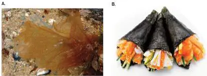
More than two membranes surround the chloroplast. The extra membranes derive from the cell membrane of the engulfed alga.
Metabolism of secondary algae includes heterotrophy. By contrast, the primary algae are near-obligate autotrophs, catabolizing only the simplest substrates, such as acetate. Several major groups of secondary algae are stramenopiles (under SAR). These include the diatoms (Bacillariophyceae); the brown algae (Phaeophyceae), such as kelps; the golden algae (Chrysophyceae), mainly flagellates; and the yellow-green algae (Xanthophyceae). The gold and yellow colors of these algae come from fucoxanthin, a light-harvesting pigment that contributes to photosynthesis. Flagellated stramenopiles generally show a pair of flagella that differ in shape. Typically, the flagellum that drives the cell through the environment is brush-like with lateral hairs, while the other is usually shorter and sometimes missing altogether. In some cases it functions like a rudder.
Diatoms (Bacillariophyceae). Diatoms are unicellular algae found ubiquitously in both fresh and marine waters (Fig. 20.28). They conduct a fifth of all photosynthesis on Earth, and they fix as much biomass as all the terrestrial rain forests. A diatom grows a unique kind of bipartite shell called a frustule. The frustule is composed of silica (cross-linked silicon dioxide, SiO 2). The silicate frustules protect diatoms from many kinds of predators. Diatoms are nonetheless consumed by flagellates and amphipods (shrimplike invertebrates) and are infected by viruses.
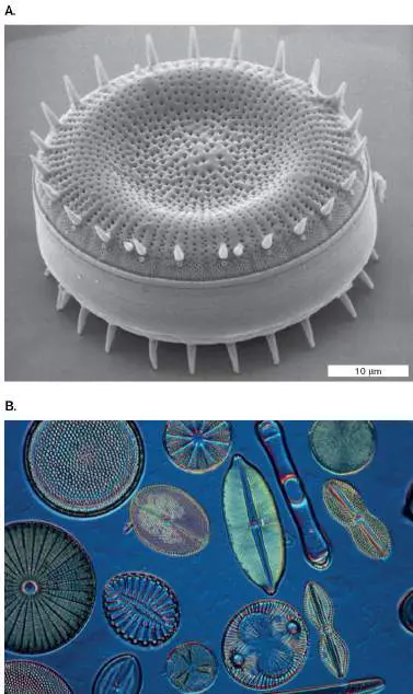
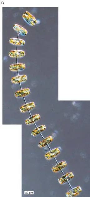
Stephanodiscus astraea, a centric diatom. B. Diverse centric and pennate diatoms. C. Chain of disk-shaped centric diatoms, Thalassiosira rotula.
BIOPHOTO ASSOCIATES/GETTY IMAGES
JAN HINSCH/SCIENCE SOURCE
MARIA PANCIC ET AL. 2018. BIOL. REV. 93 :1269, FIG. 1G
Frustules of different species form an extraordinary range of shapes with intricate pore formations (Fig. 20.28A). The shapes fall into two classes: centric, with radial symmetry; or pennate, with bilateral symmetry (Fig. 20.28B ). Spectacular chains of diatoms can be found, such as the disk-shaped diatoms shown in Figure 20.28C . Frustules of decomposed diatoms eventually sediment on the ocean floor, where they build sedimentary rock strata more than a kilometer thick. This “diatomaceous earth” is used in insulation material and in toothpaste. Diverse species of diatoms are highly sensitive to environmental factors such as pH, and the frequency of their shells in sediment can be used to track a lake’s environmental history.
Diatoms pose a unique challenge to cell division (Fig. 20.29). As the diatom grows and fissions, each daughter cell receives one parental half of the frustule while forming a new half fitting within the parental half, like the bottom dish of a Petri plate. Thus, each generation results in an inexorable decline in size of the organism. As its cell size reaches a critical point, the diatom must undergo meiosis to generate gametes. Maria Vernet at the Scripps Institution of Oceanography studies diatoms of the polar oceans, such as the Antarctic diatom Corethron criophilum. Centric diatoms such as Corethron form egg cells and flagellated sperm. When the gametes fuse, they form a special kind of zygote called an auxospore. The auxospore generates a frustule of the same size as the original diatom.
FIGURE 20.29 ■ Life cycle of a centric Antarctic diatom, Corethron criophilum. Each vegetative cell division requires formation of an in-fitting frustule half. Successive divisions result in progressive decrease in size. At a critical size limit, the diatom must undergo meiosis to form eggs and sperm. As gametes fuse, they form an auxospore, which regenerates a frustule of the original size.
WIM VAN EGMOND/SCIENCE SOURCE
Brown algae (Phaeophyceae). Kelps are familiar to ocaen bathers as the long, dark brown blades that root near the beach until the surf rips the blades off and tosses them ashore. Kelps support important communities of multicellular organisms known as kelp forests. Another type of marine “forest” consists of the unrooted sargassum weeds that float on the Sargasso Sea, a region of the Atlantic Ocean. Sargassum consists of stalks with photosynthetic blades and round gas bladders to keep the organism afloat (Fig. 20.30A). Sargassum supports a complex food web of invertebrate and vertebrate animals, including worms, crabs, fish, and sea turtles.
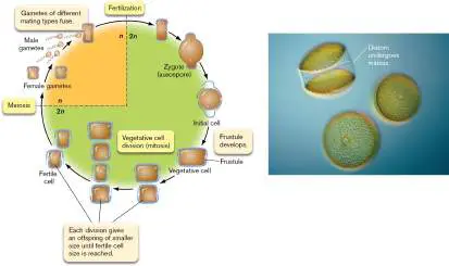
FIGURE 20.30 ■ Sargassum forests. A. Sargassum natans is the basis of the Sargasso Sea. The brown alga forms stalks with leaflike blades and round gas bladders to keep the alga afloat. Sargassum forests support animals such as the sea turtle. B. Sargassum blooms have long been concentrated in the Sargasso Sea, but a new population now stretches across the Atlantic from the Caribbean to northern Africa. Inset: Brian Lapointe, Florida Atlantic University, studies sargassum.
MASA USHIODA/VISUALS UNLIMITED
BRIAN LAPOINTE
The overgrowth of sargassum, however, can cause a problem for human communities. Rising global temperatures and nitrogen-rich
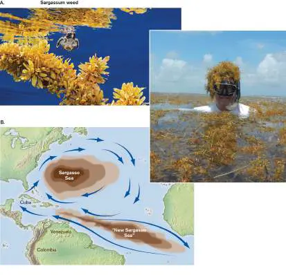
effluents have greatly expanded the Sargasso Sea—and have even generated a new band of sargassum stretching across the Atlantic as far as North Africa (Fig. 20.30B ). This expanse of sargassum now extends to the Caribbean Sea, where it piles up upon pristine beaches.
Secondary Algae: Coccolithophores
Coccolithophores (Prymnesiophyceae) are secondary algae of the unranked group Haptista (includes Haptophyta), now shown to be very distant from SAR (Fig. 20.4). Coccolithophores superficially resemble diatoms in that their cells have a mineral exoskeleton (Fig. 20.31). Instead of silicate, however, their exoskeleton is composed of calcium carbonate (CaCO 3). The calcium carbonate grows in multiple scales (unlike the bipartite exoskeleton of a diatom). The scales may extend radially in all directions, such as the “trumpet” shapes of Discosphaera tubifera (Fig. 20.31A), or they may form layers of interlocking flat, oval plates that encase the cell (Fig. 20.1A), as in Emiliana huxleyi. These scales are the “coccoliths” that give coccolithophores their name. The calcium carbonate scales protect the tiny cell from some predators.
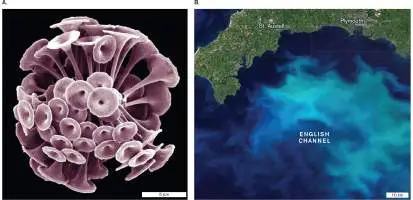
FIGURE 20.31 ■ A coccolithophore can cause marine algal blooms. A. The tiny cell Discosphaera tubifera is surrounded by a much larger volume of trumpet-shaped coccoliths. From the Alboran Sea, western Mediterranean. B. A bloom of coccolithophores fills the English Channel. The bloom appears milky white because of the calcium carbonate coccoliths (shell plates).
TRUSTEES OF THE NATURAL HISTORY MUSEUM, LONDON
NASA EARTH OBSERVATORY IMAGE BY JOSHUA STEVENS
Coccolithophores are increasingly recognized as major players in the ocean’s carbon cycle (discussed in Chapter 22). They sequester large amounts of carbon from CO 2 into their carbonate shells. Coccolithophores such as E. huxleyi generate huge blooms that appear in NASA satellite images (Fig. 20.31B ). Light reflected by their calcium carbonate appears milky white. The blooms are dissipated by predation or by virus infection.
Unfortunately, their carbonate plates are sensitive to acidification caused by the global rise in CO 2. For this reason, intensive research is focused on understanding the response of coccolithophores to pH change. In 2011, a large-scale study conducted by several European universities concluded that increasing CO 2 levels correlate with a decline in the overall mass of marine coccoliths.
To Summarize
Chlorophyta (green primary algae) contain green chloroplasts that derive from a single ancestral endosymbiosis of a cyanobacterium. Green algae include unicellular, filamentous, and sheet forms. They offer models for research on the evolution of multicellularity.
Rhodophyta (red primary algae) derive from the same ancestral endosymbiosis as green algae, and they possess the accessory photopigment phycoerythrin.
Phycoerythrin absorbs green light that is missed by green algae. Red algae include diverse seaweeds, many of which are edible for humans.
Secondary algae derive from ancestral protists that engulfed primary algae. Many are mixotrophs, combining phototrophy and heterotrophy.
Diatoms (Stramenopiles) have two-part silicate shells called frustules. Diatoms replicate by an unusual division cycle generating successively smaller frustules.
Kelps (Stramenopiles) are secondary algae that grow in long, sheetlike fronds. Kelps play an important role in the ecology of the coastal ocean, as well as the ecology of marine beaches.
Coccolithophores (Haptista or Haptophyta) are covered by calcium carbonate scales. They sequester large amounts of carbon and form algal blooms in the ocean.
Glossary
phytoplankton Phototrophic marine bacteria, algae, and protists, the primary producers in pelagic food webs.
lichen A simple multicellular organism formed by a mutualistic relationship between a fungus and an alga or cyanobacterium. cryptogamic crust A low-growing desert ground cover composed of cyanobacteria, lichens, and nonlichenous algae, fungi, and mosses.
diatom A member of the eukaryotic group Bacillariophyceae—protists that possess intricate bipartite shells that contain silica. frustule The silica bipartite shell produced by a diatom.
sargassum weed An unrooted secondary-endosymbiont form of algae that floats in marine water and forms kelp forests.
coccolithophore Marine secondary algae of the Haptista, possessing round scales of calcium carbonate.
Fig. 20.6 FIGURE 20.6 ■ Chloroplast evolution: primary and secondary endosymbiosis. A. Green algae (Chlorophyta) and red algae (Rhodophyta) contain chloroplasts (green) that evolved from engulfed cyanobacteria. B. Cryptophyte (cryptomonad) algae contain chloroplasts (green); cryptophyte secondary-host cytoplasm (yellow); and a vestigial nucleus, or nucleomorph (purple), from the engulfed primary endosymbiont. C. Marine cryptomonad, Rhodomonas salina (colorized SEM), shows double flagella.
DENNIS KUNKEL MICROSCOPY/SCIENCE SOURCE
Fig. 20.4
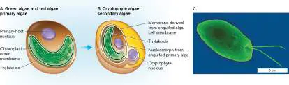
FIGURE 20.4 ■ Eukaryotic phylogeny. A phylogenetic tree of major clades (supergroups) of eukaryotes based on DNA sequence data. Dotted lines denote uncertain lineage. Green asterisks denote secondary algae whose ancestor engulfed a primary alga with chloroplast.
Sources: Modified from Sandra L. Baldauf. 2003. Science 300 :1703; and Fabien Burki et al. 2020. Trends Ecol. Evol. 35 :43.
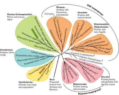
20.5 Alveolates: Ciliates, Dinoflagellates, and Apicomplexansnot assigned
The Alveolata include voracious predators such as the ciliated protists (Fig. 20.32A), as well as a major group of algae, and perhaps the most successful group of parasitic microbial eukaryotes. Alveolates are named for the flattened vacuoles called alveoli (singular, alveolus) within the cell’s outer cortex, just beneath the plasma membrane (Fig. 20.32B ; see also Fig. 20.7A). Some alveoli contain stiff plates of protein, polysaccharide, or minerals. Besides alveoli, most alveolate protists possess other kinds of cortical organelles, such as extrusomes for delivery of enzymes or toxins, bands of microtubules for reinforcement, and whiplike cilia or flagella. The alveolate cell form is highly structured, in contrast to the amorphous shape of amebas. Major groups of alveolates include ciliates, dinoflagellates, and apicomplexans.
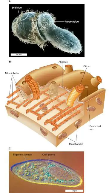
FIGURE 20.32 ■ Ciliated protists. A. Didinium, consuming Paramecium (SEM). B. Cortical structure of a ciliate. Beneath the outer cell membrane lie flattened sacs called alveoli. The cilia, composed of [9(2) + 2] microtubules, are rooted in a complex network of microtubules. Parasomal sacs take up nutrients and form endocytic vesicles. C. A Paramecium has digestive vacuoles and an oral groove for ingestion (differential interference contrast, colorized).
BIOPHOTO ASSOCIATES/SCIENCE SOURCE
M. I. WALKER/SCIENCE SOURCE
Ciliates
Alveolates of a diverse group known as Ciliophora, or ciliates, possess large numbers of cilia, short projections containing [9(2) + 2] microtubules (see eAppendix 2). Their whiplike action is driven by ATP (for review, see eAppendix 2). The cilia beat in coordinated waves that maximize the efficiency of motility. Cilia serve two functions: Cell propulsion. Coordinated waves of beating cilia, usually covering the cell surface, propel the cell forward.
Food acquisition. By generating water currents into the mouth of the cell, a ring or spiral of cilia around the mouth brings food into the cell.
Ciliate cell structure. Paramecium is one of the most studied ciliates. Paramecia feed on bacteria and in turn are consumed by other ciliates, such as Didinium (Fig. 20.32A). They can also take up smaller particles through endocytosis by specialized pores in their cortex, called parasomal sacs (Fig. 20.32B ).
The cell structure of Paramecium includes an oral groove for uptake of food driven by the beating cilia (Fig. 20.32C ). Once ingested through the oral groove, a food particle travels within the digestive vacuole in a circuit around the cell. The digestive vacuole ultimately empties into the cytoproct, a specialized vacuole for the discharge of waste outside the cell. Paramecia maintain osmotic balance by means of a contractile vacuole, a vacuole that withdraws water from the cytoplasm and then contracts while expelling it outside the cell. In this way, the cell balances the continual osmotically driven influx of water into the cytoplasm. Contractile vacuoles are widespread among protists and algae, but their mode of action has been most studied in paramecia.
Genetics and reproduction. Most ciliates have a complex genetic system involving one or more micronuclei and macronuclei. The micronucleus contains a diploid set of chromosomes that undergoes meiosis for sexual exchange (a process reviewed in eAppendix 2). For gene expression, however, one of the micronuclei develops into a macronucleus that forms hundreds of copies of its DNA. The genome in the macronucleus is present in a very different organization than in the micronucleus. In the macronucleus, it is broken up into a larger number of smaller chromosomes—in extreme cases, into many thousands of different “gene-sized” chromosomes. The huge number of chromosomes corresponds to a large number of telomeres, which are regions at the ends of chromosomes. In humans, telomere shortening is associated with aging; thus, ciliate macronucleus formation provides a model system for study of human aging.
In ciliates, only macronuclear genes are transcribed to RNA and translated to protein. When a ciliate reproduces asexually, the micronucleus undergoes mitosis, whereas the macronucleus divides by a different mechanism that is poorly understood. Cell division occurs across the long axis, necessitating generation of a new oral groove for the posterior daughter cell and a new cytoproct for the anterior daughter cell—again, a process poorly understood. Most ciliates are diploid and never produce haploid gamete cells. Instead, their sexual reproduction involves exchange of micronuclei. The two ciliates of a mating pair exchange haploid micronuclei by conjugation. In conjugation, two cells of opposite mating type form a cytoplasmic bridge and exchange their nuclear products of meiosis (Fig. 20.33). While the cells are connected, the micronucleus of each cell undergoes meiosis to form four haploid nuclei. Three out of four of the haploid nuclei disintegrate, as does the entire macronucleus. The haploid micronuclei then undergo mitosis, and one daughter nucleus from each of the two conjugating cells is exchanged across the cytoplasmic bridge. Each transferred nucleus then fuses with its haploid counterpart, restoring diploidy. The two cells come apart, and each recombined micronucleus fissions several times. One of the daughter micronuclei then transforms into the new macronucleus.
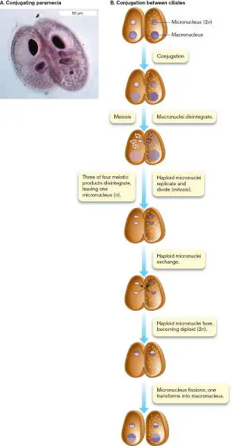
FIGURE 20.33 ■ Conjugation. A. Two paramecia conjugating (LM). B. In conjugation, two paramecia of opposite mating type form a cytoplasmic bridge. The 2 n micronucleus of each cell undergoes meiosis. Each macronucleus, as well as three out of four meiotic products, disintegrates. The haploid micronuclei undergo mitosis, forming two daughter micronuclei. Daughter nuclei from each cell are exchanged across the cytoplasmic bridge and then fuse with their respective counterparts, restoring 2 n micronuclei. The micronuclei fission several times, and one transforms into a new macronucleus.
MICHAEL ABBEY/VISUALS UNLIMITED
Thought Questions
20.9 Compare and contrast the process of conjugation in ciliates and bacteria (see Chapter 9).
20.10 For ciliates, what are the advantages and limitations of conjugation, as compared with gamete production?
Adherent ciliates. Some ciliates adhere to a substrate and use their cilia primarily to obtain prey. The cell body may be elongated or have a stalk for attachment. Ciliates such as Stentor and Vorticella have a ring of cilia surrounding a large mouth (Fig. 20.34A). The ciliary beat is specialized to draw large currents of water and whatever prey it carries. Stalked ciliates are commonly found in pond sediment and in wastewater during biological treatment by microbial digestion, where they are attached to flocs of filamentous bacteria.
FIGURE 20.34 ■ Ciliates attached to a substrate. A. Stentor, a trumpet-shaped ciliate attached to a substrate, 1.5– 2.0 mm in length (phase contrast). The oral ring of cilia generates currents drawing food into the mouth. B. The suctorian Acineta replaces cilia with knobbed tentacles (LM).
BLICKWINKEL/ALAMY STOCK PHOTO
GREG ANTIPA/SCIENCE SOURCE
Another group of stalked ciliates, the suctorians (Fig. 20.34B ), possess cilia for only a short period after a daughter cell is released by the stalked cell. The daughter cell swims by ciliary motion until it finds a good habitat in which to settle, whereupon its cilia are replaced by knobbed tentacles similar to the filopodia of shelled amebas. Suctorians prey on swimming ciliates such as paramecia.
Dinoflagellates Are Phototrophs and Predators
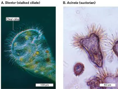
The dinoflagellates (Dinoflagellata) are a major group of marine phytoplankton, essential to marine food webs. Like ciliates, they are highly motile, but instead of numerous short cilia, dinoflagellates possess just two long flagella, one of which wraps along a crevice encircling the cell (Fig. 20.35A). Some dinoflagellates possess elaborate hornlike extensions (Fig. 20.35B ). The cell extensions increase the range of nutrient uptake, and they may deter predation.
FIGURE 20.35 ■ Dinoflagellates. A. Gymnodinium sp., a dinoflagellate, with one of its two flagella wrapped around the cell (colorized SEM). B. Ceratium sp., dinoflagellates with “horns.” C. Diagram of a dinoflagellate. Protective plates of polysaccharides are formed within cortical alveoli. The chloroplast is surrounded by a triple membrane. D. “Red tide,” caused by a bloom of dinoflagellates.
DR. DAVID M. PHILLIPS/VISUALS UNLIMITED
DENNIS KUNKEL MICROSCOPY/SCIENCE SOURCE
BILL BACHMAN/SCIENCE SOURCE
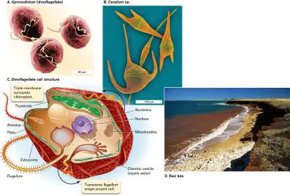
Dinoflagellates are secondary or tertiary algae. They have a chloroplast derived from a red alga, which in some species was later replaced by a heterokont alga, itself a secondary alga (Fig. 20.35C ). Some dinoflagellates possess carotenoid pigments that confer a red color. Blooms of red dinoflagellates cause the famous red tide, which may have inspired the biblical story of the plague in which water turns to blood (Fig. 20.35D ). Dinoflagellates release toxins that can be absorbed by shellfish, poisoning consumers.
The armor-plated appearance of a dinoflagellate results from its stiff alveolar plates, composed of cellulose (Fig. 20.35C ). The complex outer cortex includes various extrusomes (organelles that extrude a defensive substance) and endocytic pores, as well as a species-specific pattern of alveolar plates. Dinoflagellates supplement their photosynthesis by predation, extending a special type of pseudopod to engulf prey. Many dinoflagellates have evolved to lose their chloroplasts altogether, becoming obligate predators or parasites.
Some dinoflagellates inhabit other organisms as endosymbionts, providing sugars from photosynthesis in exchange for a protected habitat. Their hosts include shelled amebas, as well as cnidarian animals: sponges, sea anemones, and, most important, reef-building corals. Coral endosymbionts, such as zooxanthellae, are vital to reef growth. Most zooxanthellae are dinoflagellates of the family Symbiodiniaceae, including the genus Symbiodinium. The symbiotic algae are taken up by the coral’s gastrodermal cells, which enclose each dinoflagellate in an intracellular vacuole called a symbiosome (Fig. 20.36A). The vacuole enables the dinoflagellate to transfer products of photosynthesis to the host coral cell. In return, the host cell provides ammonium excreted from catabolism. Ammonium and nitrate are then used by the dinoflagellate to synthesize amino acids— something the host coral cannot do. Thus, the Symbiodiniaceae provide essential nutrients to the coral while receiving a home protected from predators.
FIGURE 20.36 ■ Symbiodinium: endosymbiotic dinoflagellate partners of coral. A. SEM micrograph of freeze-fractured internal mesentery from a reef coral polyp ( Porites porites) that shows the distribution and density of
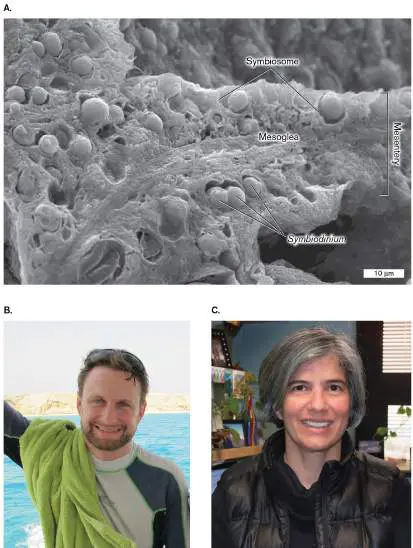
symbiont cells in host cell vacuoles. Symbiosomes are vacuoles within a gastrodermal cell. Each symbiosome contains one algal cell, which exchanges products of photosynthesis with organic nutrients from the host cell. B, C. Todd LaJeunesse and Mónica Medina study coral ecology and the effects of global climate change.
COURTESY OF TODD LAJEUNESSE
COURTESY OF TODD LAJEUNESSE
COURTESY OF MONICA MEDINA
The coral symbiosis with Symbiodiniaceae is highly sensitive to temperature. Rising temperatures in the ocean lead to coral bleaching (the expulsion of zooxanthellae), after which the coral dies. Thus, the health of coral reefs, and of large-scale ecosystems such as Australia’s Great Barrier Reef, is endangered by global climate change. Todd LaJeunesse and Mónica Medina (Fig. 20.36b and C ), at Penn State University, study the ecology of the coral-Symbiodiniaceae mutualism, and the effects of climate warming. They have found that the thylakoids (photosynthetic membranes) of the endosymbiont algae melt at higher temperatures, and that different species show widely different tolerances to heat. Within algal species, there is a lot of genetic variation, and their physiological thermal tolerance ranges are diverse. Many symbionts have local adaptations, and the host-algal combination will determine the survival of each coral population in a warming climate. eResearch Activity 20 describes experimental adaptation of coral symbionts for thermal tolerance.
Apicomplexans Are Specialized Parasites
Apicomplexans include many human parasites, such as the intestinal parasite Cryptosporidium, which infects 750,000 people annually in the United States. Apicomplexan cells have an apical complex, a highly specialized structure that facilitates entry of the parasite into a host cell. Another important apicomplexan is Toxoplasma gondii, a parasite commonly carried by cats and transmissible to humans, where it can harm a developing fetus. Like the ciliates and dinoflagellates, apicomplexans possess an elaborate cortex composed of alveoli, pores, and microtubules. But as parasites, apicomplexans have undergone extensive reductive evolution, losing their flagella or cilia. Some apicomplexans, including Toxoplasma and Plasmodium, possess a unique organelle called the apicoplast, derived by genetic reduction from an endosymbiotic chloroplast. No capacity for photosynthesis remains, but the apicoplast provides one essential function in fatty acid metabolism.
The best-known apicomplexan is Plasmodium falciparum, the main causative agent of malaria, the most important parasitic disease of humans worldwide. The disease is endemic in areas inhabited by 40% of the world’s population; it infects hundreds of millions of people and kills half a million African children each year. Historically, malaria left an impact on culture: The drug quinine, used to treat it, became a common ingredient of tonic water for its bitter taste, used in cocktails.
Figure 20.37shows red blood cells in the early “ring stage” of infection and in the “schizont” stage, which eventually bursts, releasing progeny parasites. P. falciparum is carried by mosquitoes, which transmit the parasite to humans when the insect’s proboscis penetrates the skin.
FIGURE 20.37 ■ Plasmodium falciparum, a cause of malaria. Red blood cells infected with Plasmodium falciparum, which is stained purple with a dye that interacts with DNA (LM). One late-stage infected blood cell (schizont) can be seen.
ED RESCHKE/GETTY IMAGES
The transmitted parasites invade the liver and then develop into the merozoite form that invades red blood cells (Fig. 20.38). The merozoite first contacts a red blood cell with its apical complex. The apical complex contains secretory organelles called rhoptries that inject enzymes to aid entry by the parasite. The cone-like tip of the apical complex penetrates the host cell, enabling secretion of lipids and proteins that facilitate invasion. Eventually, the entire merozoite enters the host cell, leaving no traces of the parasite on the host cell surface. Thus, the internalized parasite becomes invisible to the immune system until its progeny burst out.
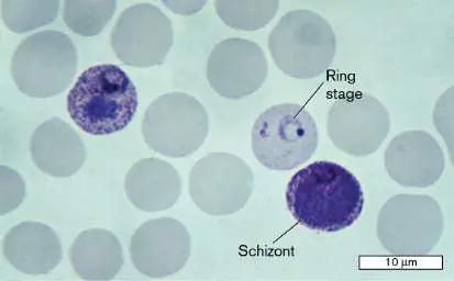
FIGURE 20.38 ■ Merozoite form of Plasmodium falciparum invades a red blood cell. The apical complex facilitates invasion and then dissolves as the merozoite transforms into an intracellular form.
P. falciparum strains have acquired resistance to drugs such as quinine, chloroquine, and artemisinin derivatives. The life cycle and molecular properties of P. falciparum have been studied extensively for clues to aid in the development of new antimalarial drugs and vaccines. The elaborate life cycle of P. falciparum and other apicomplexan parasites involves several common features:
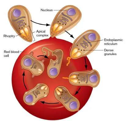
Schizogony , mitotic reproduction of a haploid form (in the mammalian host) to achieve a large population within a host tissue. Usually, the nuclei multiply first, followed by separation of individual nucleated cells.
Gamogony , the differentiation of haploid cells into male and female gametes capable of fertilization.
Mitosis and meiosis of the diploid zygote (within the insect) turns it into a haploid sporozoite form transmissible to the next host.
In the case of malaria (Fig. 20.39), whip-shaped sporozoites injected by the mosquito invade the liver, where they undergo schizogony (nuclear multiplication followed by cell separation). The cell products of schizogony are called merozoites. The merozoites from the liver then invade red blood cells, where they feed on hemoglobin. An early infected blood cell appears as a “ring stage” ( Fig. 20.37). The parasite multiplies, filling the host cell, now called a “schizont.” The schizont bursts, liberating progeny merozoites that invade another round of red cells. The bursting of red blood cells also releases cell fragments that trigger the cyclic fevers characteristic of malaria.
FIGURE 20.39 ■ Malaria: cycle of Plasmodium falciparum transmission between mosquito and human.
Some of the merozoites in the bloodstream develop into pre-gamete cells, or gametocytes. The gametocytes are acquired by bloodsucking mosquitoes and then multiply and mature (gamogony ) in the mosquito’s midgut. The gametocytes develop into female eggs and thin male cells with flagella (this is the only stage in the apicomplexan life cycle that has flagella). The male cells fertilize the egg cells, and the resulting zygotes undergo meiosis and differentiate into sporozoites, which enter the mosquito’s salivary gland for transmission to the next human host.
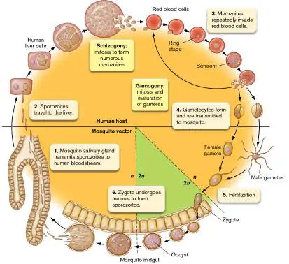
The nuclear genome of P. falciparum consists of 23 Mb contained in 14 chromosomes. Sequence annotation and expression studies predict 5,300 protein-encoding open reading frames (ORFs), comparable to the number in a yeast genome. The parasite has lost many genes encoding enzymes and transporters while expanding its repertoire of proteins involved in antigenic diversity. In addition, the parasite contains two smaller non-nuclear genomes: that of its mitochondria and that of the chloroplast-derived apicoplast. How can we treat malaria and eradicate the disease? The malarial genome reveals promising targets for drug design. For example, the fatty acid biosynthesis within the apicoplast is targeted by triclosan and other antimicrobials. Other promising targets for antimalarial drugs are the unique proteases required to digest hemoglobin within the P. falciparum food vacuole.
To Summarize
Ciliated protists (under Alveolata) are covered with numerous cilia. Cilia provide motility and help capture prey. Ciliates undergo complex reproductive cycles involving exchange of micronuclei through conjugation.
Dinoflagellates are phototrophic predators.
Dinoflagellates are tertiary endosymbiotic algae. Their alveoli contain calcified plates, and they have two very different flagella. They often prey on other eukaryotes.
Symbiodiniaceae dinoflagellates form endosymbioses with corals. Each dinoflagellate inhabits a vacuole within a coral host cell and provides products of photosynthesis. Coral bleaching (the expulsion of endosymbionts) is induced by temperature increase, a growing problem with global climate change.
Apicomplexans are parasites that penetrate host cells. The apicoplast is a specialized organ for cell invasion. Apicomplexans such as Plasmodium falciparum conduct complex life cycles within mammalian and arthropod hosts.
Glossary
oral groove A mouthlike structure of a ciliate cell, for food uptake. contractile vacuole An organelle in eukaryotic microbes that pumps water out of the cell.
micronucleus A form of nucleus found in ciliates; contains a diploid set of chromosomes and undergoes meiosis for sexual exchange by conjugation.
macronucleus A form of nucleus found in ciliates that is derived from gene amplification and rearrangement of micronuclear DNA; contains actively transcribed genes.
conjugation Horizontal gene transfer involving cell-to-cell contact. In bacteria, pili draw together the donor and recipient cell envelopes, and a protein complex transmits DNA across. In ciliated eukaryotes, a conjugation bridge forms between two cells connecting their cytoplasm, through which micronuclei are exchanged.
malaria A disease caused by the apicomplexan Plasmodium falciparum, transmitted by mosquitoes.
merozoite The form of Plasmodium falciparum, the causative agent of malaria, that invades red blood cells.
schizogony Mitotic reproduction of parasitic cells to achieve a large population within a host tissue.
gamogony The differentiation of parasitic haploid cells into male and female gametes.
Fig. 20.7A FIGURE 20.7 ■ The cortex of an alveolate contains alveoli. A. The alveolate Paramecium is covered with cilia. B. Cortex of Paramecium tetraurelia with alveoli (thin section, TEM). C. A cilium is composed of doublet microtubules enveloped in cell membrane. Flagella are similar in structure but can be much longer. D. Euplotes demonstrates ciliary motion.
Source: Part D from Danxu Tang et al. 2020. Front. Microbiol. 11:549781.
M. I. WALKER/SCIENCE SOURCE
RICHARD ALLEN (UNIVERSITY OF HAWAII) (2011)
D. TANG ET AL. 2020. FRONT MICROBIOL. 11 :549781
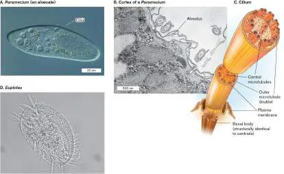
20.6 Parasitic Protozoa and Microscopic Animalsnot assigned
Many protists harmlessly inhabit the human gut as commensals. Such commensals include members of diverse clades, such as Entamoeba coli (an ameba), Blastocystis (a stramenopile), and Retortamonas intestinalis (a metamonad). Such protists may be commensal or else they might provide positive benefits to their host. Nevertheless, closely related organisms, such as Entamoeba histolytica, may cause deadly disease. The previous section introduced apicomplexan parasites of major importance, especially those that cause malaria. Other major clades of parasites (and related harmless protozoa) are the trypanosomatids, the metamonads, and amebas such as Naegleria. Finally, miniature multicellular animals (supergroup Opisthokonta, Animalia) such as mites inhabit our environment and even our bodies without our notice.
Trypanosomatids
The group Euglenida includes flagellated protists such as Euglena, with chloroplasts arising from secondary endosymbiosis. Like other algal protists, euglenas combine photosynthesis and heterotrophic nutrition. Euglenida, however, also includes a group of obligate parasites called trypanosomatids. Trypanosomatids consist of an elongated cell with a single flagellum. The cell has a unique organelle called the “kinetoplast,” consisting of a mitochondrion containing a bundle of multiple copies of its circular genome, usually placed near the base of the flagellum.
Trypanosomatids cause some of the most gruesome and debilitating conditions known to humanity, such as leishmaniasis ( Fig. 20.40A). Leishmania major (Fig. 20.40B ) causes skin infections that may enter the internal organs. If untreated, leishmaniasis can lead to swelling and decay of the extremities and eventually death. Carried by sand flies, Leishmania infects over a million people annually in South America, Africa and the Middle East, and southern Europe. Leishmania frequently infected Americans serving in Iraq; for this reason, returning veterans from Iraq have been permanently restricted from donating blood.
FIGURE 20.40 ■ Trypanosomatids. A. Patient suffering from Leishmania infection (leishmaniasis). B. Cluster of Leishmania major undergoing schizogony within the sand fly (colorized SEM). C. Trypanosoma brucei, seen here among red blood cells, is the cause of African sleeping sickness (colorized SEM).
COURTESY OF CDC/DR. D. S. MARTIN
DENNIS KUNKEL MICROSCOPY/SCIENCE SOURCE
EYE OF SCIENCE/SCIENCE SOURCE
Members of the genus Trypanosoma (called trypanosomes)
cause several major diseases, such as trypanosomiasis, also known as African sleeping sickness. The parasite Trypanosoma brucei (Fig. 20.40C ) is carried by the tsetse fly. T. brucei multiplies in the bloodstream of the host animal, causing repeated cycles of proliferation and fever. Invasion of the brain causes uncontrolled sleeping that ultimately leads to death, if untreated. This trypanosome is known for its extraordinary degree of antigenic variation. Its genome includes 200 different active versions of its variant surface glycoprotein (VSG), the antigen inducing the immune
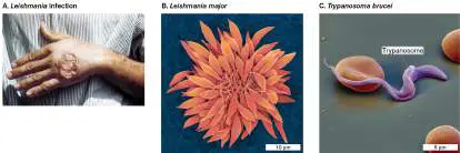
response, as well as 1,600 different “silent” versions that can recombine with “active” VSG to make further variations. In effect, the trypanosome overwhelms the host immune system by continually generating new antigenic forms until the host repertoire of antibodies is exhausted. In order to infect its human host, the trypanosome needs to interconvert among several different forms of its life cycle. The molecular basis of conversion offers targets for drug therapy.
A related trypanosome, T. cruzi, is carried by reduviid bugs, a kind of blood-feeding insect. T. cruzi causes Chagas’ disease, a debilitating infection of the heart and other internal organs. Chagas’ disease is prevalent in South and Central America, and global climate change is expected to expand its range north.
Metamonads
Metamonada is another major group of parasites and symbionts. The metamonad parasites include the diplomonads (named for their double nuclei), such as Giardia intestinalis (G. lamblia) and G. duodenalis, a common intestinal parasite (Fig. 20.41). Giardia is a frequent nemesis of day-care centers, but it also occurs in freshwater streams visited by bears and other wildlife. Giardia occasionally contaminates community water supplies in the United States and is endemic in major cities of Russia. Giardia and other metamonads are noted for their anaerobic metabolism and their modified mitochondrial organelles, reflecting their adaptation to the anaerobic intestinal environment.
FIGURE 20.41 ■ Giardia intestinalis (G. lamblia), a diplomonad flagellate and common intestinal parasite. A.
Trophozoite form of Giardia, which attaches to the intestinal epithelium (colorized SEM). B. The trophozoite form contains two nuclei, four pairs of flagella, an adhesive disk, and mitosomes (genome-less degenerate mitochondria). C. Under stress, the trophozoite encysts (differentiates into a cyst) that can survive extended periods outside the host.
Source: Parts B and C modified from Johan Ankarklev. 2010. Nat. Rev. Microbiol. 8 :413.
DR. TONY BRAIN/SCIENCE SOURCE
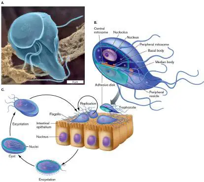
The Giardia life cycle alternates between two major forms: the trophozoite and the dormant cyst. The trophozoite (Fig. 20.41B ) has two nuclei (and, therefore, 4 n chromosomes). There are four pairs of flagella, and an “adhesive disk” enabling the parasite to adhere to the intestinal epithelium. The cell body contains no Golgi, and its mitochondria have degenerated to “mitosomes.” Mitosomes lack mitochondrial genomes. When the trophozoite experiences stress conditions, such as high levels of bile and a high pH, the organism encysts (Fig. 20.41C ). The cyst detaches from the intestine and is expelled from the host. It remains dormant until ingestion by a new host, where stomach acid triggers differentiation into a trophozoite.
Intestinal Parasites
Giardia is just one of many unpleasant intestinal visitors acquired by humans and animals. The ameba Entamoeba histolytica grows in the human colon, causing amebiasis (Fig. 20.42A). The disease includes diarrhea and possible damage to the intestinal wall; in some cases, the parasite can invade the blood and internal organs. Worldwide, E. histolytica kills tens of thousands of people per year. The organism is challenging to diagnose because it appears very similar to a harmless ameba, E. dispar, which grows normally in the intestine.
FIGURE 20.42 ■ Human intestinal protozoa. A. Entamoeba histolytica (methylene blue stain, LM). B.
Cryptosporidium parvum (colorized TEM). C. Balantidium coli (LM). D. Encephalitozoon intestinalis (TEM).
DR. GARY GAUGLER/VISUALS UNLIMITED
BIOPHOTO ASSOCIATES/SCIENCE SOURCE
CHARLES STRATTON/VISUALS UNLIMITED
LYNNE S. GARCIA. 2002. JCM 40 (6):1892–1901.
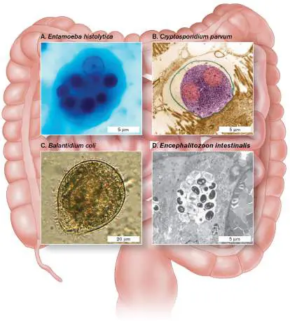
The apicomplexan Cryptosporidium parvum (Fig. 20.42B )
commonly contaminates water supplies in the United States; it caused the nation’s largest waterborne disease outbreak to date, sickening more than 400,000 people in Milwaukee in 1993.
Cryptosporidium is especially dangerous to immunocompromised patients.
An important ciliate parasite is Balantidium coli (Fig. 20.42C ). Balantidium is transmitted by a fecal-oral route, most commonly in malnourished individuals whose stomach acid is low, thus failing to kill the pathogen. Infection may be without symptoms or it can lead to diarrhea and damage the colon.
Microsporidians (Fig. 20.42D ) were once thought to be protozoa, but genetically and physiologically they are closely related to fungi (see Section 20.2). Encephalitozoon intestinalis is an obligate parasite of the intestine, causing problems especially for immunocompromised patients. More discussion of intestinal pathogens is found in Chapters 23 and 26.
Microscopic Animals
Our own clade Animalia (Opisthokonta, next to Fungi) contains all the “true” multicellular animals, from sponges to elephants—and, of course, human beings. Yet, even amidst the animals, certain forms have evolved to be so small they require a microscope to see. We all have Demodex mites (tiny arachnids) on our eyelashes that cannot be seen, and which usually cause no symptoms. Other kinds of mites cause pathology such as scabies. Invertebrate animals that cause pathology are covered in medical microbiology texts, even those that grow quite large, such as tapeworms.
Perhaps the most famous microscopic animal is the tardigrade, known informally as a “water bear” (Fig. 20.43). Their fame derives from an experiment in 2007 in which tardigrades were exposed outside a European rocket and survived travel through space vacuum and cosmic radiation. A follow-up experiment, initiated in 2021 at the International Space Station, aims to test their mechanism to survive such extreme conditions.
FIGURE 20.43 ■ Tardigrade: a microscopic free-living animal. A. A tardigrade (SEM). B. A tardigrade Echiniscus crawling on a substrate (SEM).
CULTURA RM EXCLUSIVE/GREGORY S. PAULSON/GETTY IMAGES
P. GĄSIOREK ET AL. 2019. EVOL SYST. 3 :29–39
Tardigrades possess in miniature all the major organ systems of an animal: circulation, a brain-like nerve cluster, limbs with digits, and even sucker feet. Tardigrades typically inhabit aquatic vegetation, using an oral “stylet” to pierce cells for nutrition. Evolutionary biologists consider the most likely origin of tardigrades to have been the miniaturization of a larger ancestral animal.
To Summarize
Trypanosomatids include the important parasites Leishmania (cause of leishmaniasis) and the trypanosomes Trypanosoma brucei (cause of African sleeping sickness) and Trypanosoma cruzi (cause of Chagas’ disease).
Metamonads include parasites such as Giardia intestinalis, a frequent contaminant of natural freshwater environments
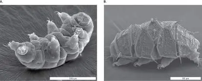
that is frequently transmitted among children.
Other intestinal parasites include the ameba Entamoeba histolytica, the apicomplexan Cryptosporidium parvum, the ciliate Balantidium coli, and the microsporidian Encephalitozoon intestinalis.
Miniature animals can be microscopic, although they are technically not considered microbes. Some are free-living, such as tardigrades, whereas others such as mites inhabit human bodies.
Glossary
trypanosomatid A parasitic excavate protist that has a cortical skeleton of microtubules culminating in a long flagellum.
tardigrade A microscopic segmented animal with eight legs, miniaturized by evolution; possesses few-celled forms of all major organ systems.
eResearch Activity 20
Can Coral Endosymbiotic Algae Adapt to Rising Heat?
Australia’s Great Barrier Reef, home to 10% of all of Earth’s corals, has a problem. Since 1995, half the corals on its 900 islands have died off by “bleaching,” the loss of algal endosymbionts that conduct photosynthesis and feed their coral hosts. The cause of the die-off is complex, but the major factor is the increase in ocean temperature —a problem that afflicts corals and other marine life worldwide (discussed in Section 20.5).
Besides affecting coral directly, the rise in temperature affects the coral’s endosymbionts, the Symbiodiniaceae dinoflagellates that inhabit coral polyps and share their products of photosynthesis. The corals have no choice about it—to survive the future, they will need to adapt. Can their endosymbionts adapt to climate change? In other words, can the algae evolve thermal tolerance and avoid coral bleaching? Madeleine van Oppen, at the University of Melbourne, Australia, aims to find out—by conducting evolution experiments on the symbiotic algae (Fig. ERA 20.1 ).
For evolution, van Oppen’s research group selected the alga Cladocopium goreaui, which inhabits the coral Acropora tenuis from Magnetic Island, Great Barrier Reef (Fig. ERA 20.1 ). This endosymbiont can be obtained from the coral and grown separately in the laboratory. A clonal population of C. goreaui was divided into subpopulations and cultured in flasks at either the high temperature (31°C) or the optimal marine temperature (27°C). The algal populations were serially subcultured for 4 years, which amounted to 120 asexual generations. The Symbiodiniaceae algae grow more slowly than Escherichia coli and other bacteria investigated by experimental evolution (see Chapter 17).
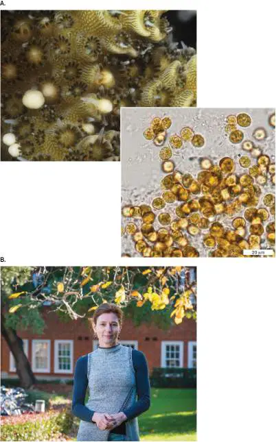
FIGURE ERA 20.1 ■ Coral with symbiotic algae evolving thermal tolerance. A. Acropora tenuis coral spawning (releasing sperm and egg packets) at Magnetic Island, Great Barrier Reef, Australia. Inset: Symbiotic dinoflagellates ( Cladocopium sp.). B. Madeleine van Oppen, Australian Institute of Marine Science, University of Melbourne.
AUSCAPE INTERNATIONAL PTY LTD/ALAMY STOCK PHOTO
K. E. TURNHAM ET AL. 2021. ISME J. 15 :3271–3285
MADELEINE VAN OPPEN
After the lengthy period of evolution, the heat-evolved algal populations were acclimated (physiologically adapted) to the lower temperature again. Samples of both heat-adapted and wild-type evolved algal cultures were then incubated again at 31°C, and their growth rates were measured. The heat-adapted algal strains grew to population sizes threefold higher than that of the wild-type algal strain. This increased growth rate was likely due to mutations that occurred during fitness selection over the 4-year period.
If the C. goreaui cells grew and proliferated outside their hosts, would the evolved populations now grow again within the coral— and continue to tolerate higher temperature? van Oppen tested this question by using the evolved alga to inoculate coral larvae. The coral host spawns once per year, with simultaneous release of sperm and egg packets (Fig. ERA 20.1A ). Once fertilization occurs, the embryos develop into larvae (also called planulae). The larvae float on ocean currents until they find a nutrient-rich location to start growing as coral. In order to grow, each larva needs to be colonized by appropriate symbiotic algae.
As shown in Figure ERA 20.2 , the researchers inoculated coral larvae with samples of each of the heat-evolved algal strains (labeled SS numbers 1–10) and with two algal strains evolved at the lower temperature (WT1 and WT2). The inoculated larvae were then exposed to marine water for 7 days at the higher temperature, 31°C. After exposure, the larvae were tested for endosymbiont retention (cells per larva) and for photosynthetic output (chlorophyll production, measured by fluorimetry).
FIGURE ERA 20.2 ■ Heat-evolved algal symbionts increase coral heat tolerance. A. Coral larvae were inoculated with heat-evolved strains of Cladocopium goreaui and incubated for 7 days at 31°C. Graph shows change in algal cell
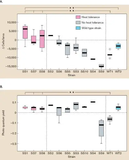
number per coral larva; numbers above zero indicate thermal tolerance and resistance to coral expulsion. B. Most of the heat-evolved strains show increased quantum yield of algal photosynthesis.
In this experiment, the coral larvae maintained three of the heat-adapted algal populations (SS1, SS7, SS8) at significantly higher levels than they maintained the wild-type algal populations (WT1, WT2). This exciting result suggests that coral endosymbionts may be capable of heat adaptation to avoid coral expulsion. In another encouraging observation, the heat-adapted algae maintained their photosynthetic production at levels comparable with those of the wild-type algae. By maintaining photosynthesis as well as thermotolerance, it is hoped that the coral-algal symbiosis can avoid bleaching and death as temperatures rise. This one small experiment offers modest hope that some corals will survive climate change—and that humans might culture heat-adapted strains to assist coral survival.
Further Exploration
Why do only certain heat-evolved algal strains maintain thermal tolerance in their coral hosts? What will happen when the coral larvae settle and start building corals? Will the coral hosts also need to evolve thermal tolerance? What about other climate changes, such as ocean acidification: Could the algae also evolve acid tolerance? What special problem is faced by dinoflagellates?
Buerger, P., C. Alvarez-Roa, C. W. Coppin, S. L. Pearce, L. J. Chakravarti, et al. 2020. Heat-evolved microalgal symbionts increase coral bleaching tolerance. Science Advances 6 :eaba2498.
CHAPTER REVIEW
Review Questions
1. Discuss the evidence for the branching of fungi and animals within one clade, the Opisthokonta, which is distinct from algae and protists.
2. How do primary symbiont algae differ from secondary and tertiary symbiont algae? Compare with respect to cell structure and nutritional options.
3. Compare and contrast the molecular basis of motility in amebas and ciliates. Cite particular species.
4. Compare and contrast kelps, diatoms, and dinoflagellates in terms of cell structure, colony organization, and nutritional options.
5. Summarize the key traits of fungi. What do fungi have in common with protists, and how do they differ?
6. Outline the life cycles of the major phyla of fungi: Chytridiomycota, Zygomycota, Ascomycota, and Basidiomycota. Explain their ecological significance. 7. Compare and contrast the traits of green and red algae. 8. Outline the life cycle of the slime mold Dictyostelium discoideum. Compare and contrast its features with those of fungi that produce fruiting bodies, such as basidiomycetes.
9. Outline the complex parasitic life cycles of an apicomplexan parasite and a trypanosomatid. Cite evidence of reductive evolution, as well as of evolution of elaborate specialized structures to facilitate the parasite’s life cycle.
Thought Questions
1. Compare and contrast eukaryotic microbes that have inorganic shells or plates. What is their composition, and how do they grow?
2. Explain mixotrophy. Why are so many marine eukaryotes mixotrophs?
3. Why do eukaryotes show such a wide range of cell size? Which selective forces favor large cell size, and what favors small cell size?
4. Do eukaryotic parasites have genomes that are larger or smaller than those of free-living organisms? Explain.
Key Terms
alga (806, 809)
alternation of generations (815) alveolate (810)
ameba (809)
apicomplexan (810)
arbuscular mycorrhizae (822) ascomycete (818)
ascospore (820)
ascus (815)
basidiomycete (821) basidiospore (822)
budding (814)
cellular slime mold (825) chlorophyte (810)
chloroplast (809)
ciliate (810)
cilium (810)
coccolithophore (834) conjugation (837)
contractile vacuole (836) cortical alveolus (810) cryptogamic crust (831) diatom (832)
dinoflagellate (810) endosymbiosis (807) Eumycota (807)
flagellate (810)
flagellum (810)
foraminiferan (827) fruiting body (807) frustule (832)
fungus (805)
gamogony (841)
green alga (810)
hypha (812)
lichen (831)
macronucleus (836)
malaria (840)
merozoite (840)
micronucleus (836)
mitosis (814)
mitosporic fungus (815) mycelium (812)
mycology (805)
mycorrhizae (822)
nucleomorph (810)
Oomycetes (824)
oral groove (836)
phagocytosis (824)
phylogenomics (807) phytoplankton (828) Plantae (Archaeplastida) (809) plasmodial slime mold (827) plasmodium (827)
primary algae (806, 809) protist (806)
protozoan (806)
pseudopod (809)
radiolarian (827)
red alga (810)
Rhizaria (809)
rhodophyte (810)
sargassum weed (833) schizogony (841)
secondary algae (806, 810) sporangiospore (818) sporangium (818)
Stramenopiles (810) tardigrade (845)
true fungi (807)
trypanosomatid (842) yeast (814)
zoospore (807)
zygomycete (818)
zygospore (818)
Recommended Reading
Ankarklev, Johan, Jon Jerlström-Hultqvist, Emma Ringqvist, Karin Troell, and Staffan G. Svärd. 2010. Behind the smile: Cell biology and disease mechanisms of Giardia species. Nature Reviews. Microbiology 8 :413–422.
Armbrust, E. Virginia. 2009. The life of diatoms in the world’s oceans. Nature 459 :185–192.
Beaufort, L., I. Probert, T. de Garidel-Thoron, E. M. Bendif, D. Ruiz-Pino, et al. 2011. Sensitivity of coccolithophores to carbonate chemistry and ocean acidification. Nature 476 :80– 83.
Burki, Fabien, Andrew J. Roger, Matthew W. Brown, and Alastair G. B. Simpson. 2020. The new tree of eukaryotes. Trends in Ecology & Evolution 35 :43–55.
Davy, Simon K., Denis Allemand, and Virginia M. Weis. 2012. Cell biology of cnidarian-dinoflagellate symbiosis. Microbiology and Molecular Biology Reviews 76 :229–261.
Fisher, Matthew C., Daniel A. Henk, Cheryl J. Briggs, John S. Brownstein, Lawrence C. Madoff, et al. 2012. Emerging fungal threats to animal, plant and ecosystem health. Nature 484 :186–194.
Genre, Andrea, Luisa Lanfranco, Silvia Perotto, and Paola Bonfante. 2020. Unique and common traits in mycorrhizal symbioses. Nature Reviews. Microbiology 18 :649–660.
Henderson, Gregory P., Lu Gan, and Grant J. Jensen. 2007. 3-D ultrastructure of O. tauri: Electron cryotomography of an entire eukaryotic cell. PLoS One 8 :e749.
Kronstad, James W., Rodgoun Attarian, Brigitte Cadieux, Jaehyuk Choi, Cletus A. D’Souza, et al. 2011. Expanding fungal pathogenesis: Cryptococcus breaks out of the opportunistic box. Nature Reviews. Microbiology 9 :193–203. LaJeunesse, Todd, John Everett Parkinson, Paul W.
Gabrielson, Hae Jin Jeong, James Davis Reimer, et al. 2018. Systematic revision of Symbiodiniaceae highlights the antiquity and diversity of coral endosymbionts. Current Biology 28 :P2570–2580.E6.
Lapointe, B. E., R. A. Brewton, L. W. Herren, M. Wang, C. Hu, et al. 2021. Nutrient content and stoichiometry of pelagic Sargassum reflects increasing nitrogen availability in the Atlantic Basin. Nature Communications 12 :1–10.
Lew, Roger R. 2011. How does a hypha grow? The biophysics of pressurized growth in fungi. Nature Reviews. Microbiology 9:509–518.
Martin, Francis, Annegret Kohler, Claude Murat, Claire Veneault-Fourrey, and David S. Hibbett. 2016. Unearthing the roots of ectomycorrhizal symbioses. Nature Reviews. Microbiology 14 :760–773.
Parfrey, Laura W., and Laura A. Katz. 2010. Dynamic genomes of eukaryotes and the maintenance of genomic integrity. Microbe 5 :156–163.
Pounds, J. Alan, Martin R. Bustamante, Luis A. Coloma, Jamie A. Consuegra, Michael P. L. Fogden, et al. 2007. Widespread amphibian extinctions from epidemic disease driven by global warming. Nature 439 :161–167.
Ratcliff, William C., Matthew D. Herron, Kathryn Howell, Jennifer T. Pentz, Frank Rosenzweig, et al. 2013.
Experimental evolution of an alternating uni-and multicellular life cycle in Chlamydomonas reinhardtii. Nature Communications 4 :2742.
Wahlgren, Mats, Suchi Goel, and Reetesh R. Akhouri. 2017. Variant surface antigens of Plasmodium falciparum and their roles in severe malaria. Nature Reviews. Microbiology 15 :479– 491.
Glossary
Stramenopiles Also called Heterokonta. A superphylum of eukaryotic microbes that usually possess a pair of differently shaped flagella. sporangium pl. sporangia A fungal organ that releases nonmotile spores.
sporangiospore A haploid spore of a fungus that can germinate to form a haploid mycelium.
secondary algae Algae that evolved by engulfing primary algae in a second endosymbiotic event.
schizogony Mitotic reproduction of parasitic cells to achieve a large population within a host tissue.
sargassum weed An unrooted secondary-endosymbiont form of algae that floats in marine water and forms kelp forests.
rhodophyte See red alga .
Rhizaria A clade of eukaryotic microbes that have filamentous pseudopods.
red alga Also called rhodophyte. An alga of the eukaryotic group Rhodophyta, which contain chloroplasts as primary algae, with red accessory photopigments.
radiolarian A member of the eukaryotic group Radiolaria—amebas with a silicate shell penetrated by filamentous pseudopods. pseudopod A locomotory extension of cytoplasm enclosed by the cell membrane.
protozoan pl. protozoa A heterotrophic eukaryotic microbe, usually motile, that is not a fungus.
protist A single-celled eukaryotic microbe, usually motile; not a fungus. primary algae Algae that are derived from a single endosymbiotic event; closely related to green plants (Plantae).
plasmodium pl. plasmodia The giant, multinucleate cell formed by a plasmodial slime mold.
plasmodial slime mold A slime mold in which a fertilized zygote undergoes multiple nuclear divisions, generating a multinucleate single cell (plasmodium).
Plantae Also called Archaeplastida. A eukaryotic superphylum that includes plants, as well as green and red primary algae. phytoplankton Phototrophic marine bacteria, algae, and protists, the primary producers in pelagic food webs.
phylogenomics The construction of phylogenetic trees of related clades on the basis of comparison of whole genomes.
phagocytosis A form of endocytosis in which a large extracellular particle is brought into the cell.
oral groove A mouthlike structure of a ciliate cell, for food uptake. Oomycetes Formerly called water molds. A member of the eukaryotic group Oomycetes—heterokont protists whose life cycle resembles that of fungi; formerly classified as fungi (Oomycota).
nucleomorph A vestigial nucleus within a eukaryotic cell, evolved by genetic reduction from the nucleus of an endosymbiont.
mycorrhizae sing. mycorrhiza Fungi involved in an intimate mutualism with plant roots, in which nutrients are exchanged.
mycology The study of fungi.
mycelium pl. mycelia A single mass of fungal hyphae that projects into the air (aerial mycelium) or into the growth substrate (surface mycelium). mitosporic fungus Also called imperfect fungus. A species of fungus that generates spores by mitosis and lacks a known sexual cycle. mitosis The orderly replication and segregation of eukaryotic chromosomes, usually prior to cell division.
micronucleus A form of nucleus found in ciliates; contains a diploid set of chromosomes and undergoes meiosis for sexual exchange by conjugation.
merozoite The form of Plasmodium falciparum, the causative agent of malaria, that invades red blood cells.
malaria A disease caused by the apicomplexan Plasmodium falciparum, transmitted by mosquitoes.
macronucleus A form of nucleus found in ciliates that is derived from gene amplification and rearrangement of micronuclear DNA; contains actively transcribed genes.
lichen A simple multicellular organism formed by a mutualistic relationship between a fungus and an alga or cyanobacterium. hypha pl. hyphae The threadlike filament that forms the mycelium of a fungus. green alga Also called chlorophyte. A member of the eukaryotic group Chlorophyta—microbes that have chloroplasts; closely related to plants (Plantae).
gamogony The differentiation of parasitic haploid cells into male and female gametes.
fungus pl. fungi A heterotrophic opisthokont eukaryote with chitinous cell walls. Includes Eumycota, but traditionally may refer to fungus-like protists such as the oomycetes.
frustule The silica bipartite shell produced by a diatom.
fruiting body A multicellular fungal or bacterial reproductive structure. foraminiferan or foram An ameba with a calcium carbonate shell and a helical arrangement of chambers.
flagellum pl. flagella A filamentous structure for motility. In prokaryotes, a helical protein filament attached to a rotary motor; in eukaryotes, an undulating membrane-enclosed complex of microtubules and ATP-driven motor proteins.
flagellate A protist that has one or more flagella.
Eumycota True fungi, a taxonomic group of opisthokont eukaryotes with chitinous cell walls; the group most closely related to animals. endosymbiosis An intimate association between different species in which one partner population grows within the body of another organism. dinoflagellate A member of the eukaryotic group Dinoflagellata—secondary or tertiary endosymbiont algae, alveolates with two flagella, one of which is wrapped distinctively around the cell equator. diatom A member of the eukaryotic group Bacillariophyceae—protists that possess intricate bipartite shells that contain silica. cryptogamic crust A low-growing desert ground cover composed of cyanobacteria, lichens, and nonlichenous algae, fungi, and mosses.
cortical alveolus One of the vesicles that forms a network in the outer covering of an alveolate protist.
contractile vacuole An organelle in eukaryotic microbes that pumps water out of the cell.
conjugation Horizontal gene transfer involving cell-to-cell contact. In bacteria, pili draw together the donor and recipient cell envelopes, and a protein complex transmits DNA across. In ciliated eukaryotes, a conjugation bridge forms between two cells connecting their cytoplasm, through which micronuclei are exchanged.
coccolithophore Marine secondary algae of the Haptista, possessing round scales of calcium carbonate.
cilium pl. cilia A short, hairlike structure of eukaryotes that is structurally similar to the prokaryotic flagellum. Cilia beat in waves to propel the cell.
ciliate An alveolate that has paired cilia.
chloroplast An organelle of endosymbiotic origin (sharing descent with cyanobacteria) that conducts oxygenic photosynthesis; found in algae and plant cells.
chlorophyte See green alga .
cellular slime mold A slime mold in which the individual bacterial cells retain their own cell membranes; not a fungus.
budding A form of reproduction in which mitosis of the mother cell generates daughter cells of unequal size.
basidiospore A haploid spore formed by a basidiomycete through meiosis of a basidium, a reproductive cell of a mushroom.
basidiomycete A member of the eukaryotic group Basidiomycota—fungi that form mushrooms.
ascus pl. asci A spore-containing pod produced by ascomycete fungi. ascospore The spore produced by an ascomycete fungus.
ascomycete A member of the eukaryotic group Ascomycota—fungi whose mycelia form paired nuclei. Haploid ascospores are produced in pods called asci.
arbuscular mycorrhizae Also called vesicular-arbuscular mycorrhizae or endomycorrhizae. Mutualistic associations between plant roots and certain fungi, involving hyphal penetration of plant root cells.
apicomplexan A member of the eukaryotic group Apicomplexa—parasitic alveolates that possess an apical complex used for entry into a host cell.
ameba or amoeba A protist that moves via pseudopods.
alveolate A member of the eukaryotic group Alveolata—ciliated or flagellated protists with complex cortical structure. alternation of generations A life cycle that alternates between populations of haploid cells and diploid cells, which undergo meiosis and fertilization. alga pl. algae A microbial eukaryote that contains chloroplasts.
tardigrade A microscopic segmented animal with eight legs, miniaturized by evolution; possesses few-celled forms of all major organ systems.
zygospore In zygomycetes, the diploid structure formed by the fusion of two gamete-bearing hyphae.
zygomycete A member of the eukaryotic group Zygomycota—fungi forming nonmotile haploid gametes that grow toward each other, fusing to form the zygospore.
zoospore A flagellated reproductive cell produced by chytridiomycete fungi.
yeast A unicellular fungus.
trypanosomatid A parasitic excavate protist that has a cortical skeleton of microtubules culminating in a long flagellum.
true fungi See Eumycota .