Chapter introduction
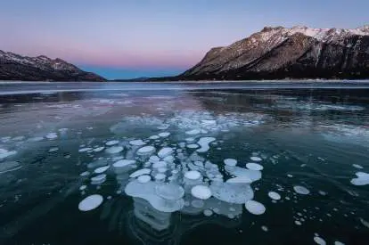
Trapped methane bubbles at Lake Abraham, Alberta, Canada. Below the lake in anoxic sediment, methanogenic archaea convert carbon dioxide and bacterial fermentation products into methane. Methane is a potent greenhouse gas, and its release from warming lakes and thawing tundra accelerates the rise of global temperature.
Microbes throughout the biosphere recycle carbon, nitrogen, and other elements essential for all life. Through their biochemical transformations, diverse microbial activities largely determine the quality of soil, air, and water. Today, all of these geochemical cycles In Chapter 22, we show how the collective metabolic activities of microbial populations generate global cycles of elements throughout Earth’s biosphere. Gases such as CO 2 trap solar radiation and release it as heat in a phenomenon known as the greenhouse effect. Greenhouse gases are generated by bacteria, methanogenic archaea, and other life forms. But human technology accelerates the release of greenhouse gases at a rate that the planet’s ecosystem never evolved to tolerate. As snow and ice melt earlier each spring, the associated growth of microbes may, in turn, accelerate the melting and warming. Will the human-induced global climate change cause mass extinctions of Earth’s species—as did the rise of ancient cyanobacteria producing oxygen? Or can we use our knowledge of microbial ecology to channel microbial activities into recovering the balance; for example, by increasing microbial CO 2 fixation?
On a more local level, we consider the role of microbial communities in our human-built environment. The built environment consists of human-made constructs that we inhabit on a daily basis, from our homes to our workplaces and parks. Our many microbial inhabitants, from lactococci to coronavirus, influence our health for good or ill. The concept of our built environment expands as we recognize the growing impact of human activity throughout the biosphere. Microbes can help us manage environmental change both locally and globally. From wastewater treatment to the control of greenhouse gases, microbes are our hidden partners on Earth. Earth’s microbial cycles lead us to wonder whether biospheres exist on other worlds. The highly speculative field of astrobiology addresses this question. The one place left where life may remain untouched by humans is other planets, if life exists there.
Glossary
built environment Buildings and other human-built constructs that humans inhabit or use for work and recreation.
22.1 The Carbon Cycle and Climate Changenot assigned
Microbes acquire their elements either from nonliving components of their environment, such as by fixing atmospheric CO 2, or from other organisms, by grazing, predation, or decomposition. Furthermore, all organisms recycle their components back to the biosphere. The partners in this recycling include abiotic entities such as air, water, and minerals, as well as biotic entities such as predators and decomposers. All elements used for life flow in biogeochemical cycles of nutrients throughout the biotic and abiotic components of the biosphere. Collectively, the metabolic interactions of microbial communities with the biotic and abiotic components of their ecosystems are known as biogeochemistry or geomicrobiology.
Microbial Chemistry and Climate Change
Over timescales of thousands of years, the availability of life’s core elements (carbon, oxygen, and nitrogen) in the biosphere was remarkably constant. The constant level of available carbon in the atmosphere and oceans depends on the maintenance of a “steady state” in which different forms of an element (such as carbon in CO 2 molecules versus carbon in organic compounds) are interconverted at rates that balance out. Some of these extremely important reactions —such as nitrogen fixation and oxidation, and methane production and oxidation—depend entirely on microbes. Carbon dioxide fixation depends entirely on microbes and the chloroplasts of plants.
Over the past three centuries, however, Earth’s cycles of carbon and nitrogen have been drastically altered by human technology. Most prominently, the burning of fossil fuels transfers terrestrial carbon into the atmosphere, and the result of our activity has been a rapid rise in the concentrations of the greenhouse gases carbon dioxide, methane, and nitrous oxide (Fig. 22.1A). The greenhouse effect describes how these gases allow light rays to penetrate the atmosphere but block lower-energy heat radiation from leaving the planet. Some degree of a greenhouse effect is necessary for life; without it, our planet might look more like Mars. But if Earth’s temperature increases faster than heat can radiate out, the planet might instead turn into something more like Venus, too hot for life. In 2019, the United Nations Environment Programme found that greenhouse gas emissions need to decrease by half in order to avoid a global temperature increase with potentially catastrophic effects on the planet. Concerns raised by scientific reports on climate change have inspired an international youth movement led by people such as Swedish activist Greta Thunberg (Fig. 22.1B ).
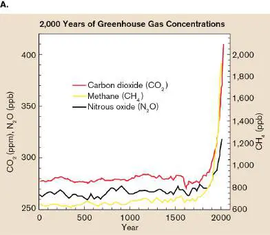
FIGURE 22.1 ■ Global greenhouse gases. A. Atmospheric levels of CO 2, methane, and nitrous oxide were measured in Antarctic ice cores. The increase of these greenhouse gases since 1750 accompanies the rise in fossil fuel burning and fertilizer-intensive agriculture. B. At the United Nations Climate Action Summit, young activist Greta Thunberg demanded that world leaders take action to halt carbon emissions. Source: Part A modified from U.S. Global Change Research Program. 2009. Global Climate Change Impacts in the United States. Cambridge University Press.
UPI/ALAMY STOCK PHOTO
Sources and Sinks of Elements

The challenge of studying biogeochemical cycles is quantification— how to add up all the inputs and outputs of key molecules on a global scale. The parts of the biosphere that contain major amounts of an element needed for life are called reservoirs (Fig. 22.2). Each reservoir acts both as a source of that element for living organisms and as a sink to which the element returns. The transfer of elements between sources and sinks, via biotic and abiotic processes, forms the global biogeochemical cycles. In all of these cycles, key parts are played by microbes.
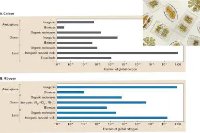
FIGURE 22.2 ■ Global reservoirs of carbon and nitrogen. A. The largest reservoir of carbon is Earth’s crust, but carbon cycles through the biosphere extremely slowly. The major reservoirs for cycling are marine inorganic carbon (CO 2 and carbonates), atmospheric CO 2, and buried fossil fuels. Inset: Marine phytoplankton fix much of Earth’s CO 2. B. The largest reservoirs of nitrogen are atmospheric N 2 and Earth’s crust. Numbers represent the proportion of total global carbon and nitrogen, respectively.
Source: Part B modified from R. Maier et al. 2000. Environmental Microbiology.
Academic Press.
ELIF BAYRAKTAR/SHUTTERSTOCK
The rate of cycling between sources and sinks determines the importance of a reservoir for the biosphere. For example, in theory, carbonate rock forms the largest reservoir of carbon (Fig. 22.2A). But Earth’s crust is the source least accessible to the biosphere as a whole. Crustal rock provides carbon only to organisms at the surface and to subsurface microbes that grow extremely slowly. Thus, subsurface carbon turnover is very slow. The carbon reservoir that cycles most rapidly is that of the atmosphere, a source of CO 2 for photosynthesis and chemolithoautotrophy. The atmosphere also acts as a sink for CO 2 produced by heterotrophy and by geological outgassing from volcanoes.
For the biosphere, the major source of carbon (CO 2 in equilibrium with HCO −, bicarbonate ion) is the ocean. Ocean carbon cycles
3
with CO 2 in the atmosphere. The dissolving of atmospheric CO 2 into marine water is the most important abiotic portion of the carbon cycle. Biotic cycling occurs when organotrophs release CO 2 into the atmosphere and when phototrophs and lithotrophs fix CO 2. Marine phytoplankton (photosynthetic bacteria and algae) fix an extraordinary amount of CO 2 into biomass; for example, diatoms alone fix as much carbon as all the world’s rain forests.
The atmospheric reservoir of carbon is much smaller than other sources, such as the oceans, crustal rock, and fossil fuels. For this reason, the industrial burning of fossil fuels has perturbed the balance between atmospheric CO 2 and larger reservoirs, such as the ocean. But despite the ocean’s carbon capture, atmospheric CO 2 is rising at an ever-faster rate, unprecedented in Earth’s history (Fig. 22.1A). Today, CO 2 level increases at an annual rate of 2 parts per million (ppm), which is twice the rate that was observed less than a century ago, in the 1960s. In 2022, the Mauna Loa Observatory in Hawaii measured a CO 2 level of 420 ppm—the highest level on Earth for the past 3 million years—and it continues to increase.
The relative importance of global sources and sinks varies with each element. For nitrogen (Fig. 22.2B ), Earth’s dominant source is nitrogen gas (N 2) in the atmosphere.
The only biotic processes that fix N 2 into biomass, and that return N 2 to the atmosphere, are performed by bacteria and archaea (see Section 22.3). Thus, the nitrogen cycles of all ecosystems require microbes.
Oxidation-State Changes during Carbon Flux
As elements cycle from sources to sinks, microbial metabolism generates a series of redox changes (discussed in Chapter 14). Since the planet was formed, oxidation of carbon has had a profound impact on the biosphere. Two billion years ago, ancient cyanobacteria were the first to photolyze water and produce molecular oxygen (see Chapter 17). Oxygen is a powerful oxidant, lethal to most life in that anoxic era, when all living organisms were anaerobic microbes. To survive, microbes evolved defenses such as antioxidant molecules and enzymes. Since then, microbes have shaped our biosphere by releasing oxygen, by fixing nitrogen and returning it to the atmosphere, and by fixing and producing carbon dioxide.
The major oxidation states of carbon are summarized in Table 22.1. Biospheric carbon can be found as CH 4 generated by methanogens (completely reduced, −4), as CO 2 produced by respiration and fermentation (completely oxidized, +4), or as one of various intermediate states of oxidation (carbohydrates, alcohols, acids). Near Earth’s surface, carbon is found in more oxidized states, as living organisms rapidly combine it with oxygen to yield energy. Reduced forms of carbon, such as methane and hydrocarbons (petroleum), are found buried deep underground, where oxygen gas has been unavailable for millions of years.
Oxidation States of Carbon
TABLE 22.1
Compounds
Oxidation state Carbon molecule −4 CH 4 Methane −2 CH 3 OH, (CH 2) Methanol, hydrocarbon n 0 (CH 2 O) n Carbohydrate +2 CHOOH Formic acid CO, HCO − +4 2 3 Carbon dioxide, bicarbonate ion The results of carbon cycling differ greatly, depending on the presence of molecular oxygen. Thus, the global cycle of carbon is closely linked to the cycles of oxygen and hydrogen, elements to which most carbon is bonded. Overall, carbon cycles between carbon dioxide and various reduced forms of carbon, including biomass (living material).
Thought Question
22.1 Why is oxidation state important for microbes to use and cycle compounds? Cite examples based on your study of microbial metabolism (see Chapter 14).
Experimental Measurement of Element Cycling
How do we study the cycling of elements on a global scale? How do we figure out whether ecosystems are net sources or sinks of CO 2? Does microbial activity enhance or limit availability of nitrogen? Rates of flux of elements in the biosphere are very difficult to measure, yet the questions have enormous political and economic implications. To measure environmental carbon, nitrogen, and other elements, various methods are used. These methods fall under the following categories: Chemical and spectroscopic analysis. Bulk quantities of CO 2, nitrates, and other chemicals can be determined by sophisticated chemical instrumentation. Atmospheric CO 2 is measured by infrared absorption spectroscopy, applied to samples from towers such as those of NASA’s FLUXNET study ( Fig. 22.3). Gas chromatography is used to separate and quantify various gases, including oxygen, nitrogen, sulfur dioxide, and carbon monoxide. Mass spectrometry detects extremely small quantities of different molecules, even distinguishing between elemental isotopes.
Radioisotope incorporation. The influx and efflux of CO 2 can be measured by the uptake of 14 C-labeled substrates in a small, controlled model ecosystem called a mesocosm. Alternatively, CO 2 flux can be measured with radioisotope tracers in the field by use of a field chamber.
Stable isotope ratios. Some enzyme reactions show a preference for one isotope over another, such as 14 N versus 15 N. Both isotopes are stable (nonradioactive). For example, denitrifiers (bacteria that metabolize nitrate) strongly prefer the 14 N isotope, leaving behind nitrate enriched in 15 N. The 14 N/ 15 N ratio is measured using mass spectrometry. Measuring nitrogen isotope ratios can indicate whether denitrifiers could have conducted metabolism in the sample. Further examples of stable-isotope analysis are presented in Chapter 17.
FIGURE 22.3 ■ Measuring flux of elements in the biosphere. A. A U.S. FLUXNET tower at Tonzi Ranch, California, is used for atmospheric CO 2 sampling as part of a global effort to monitor carbon flux. B. Peak CO 2 uptake by forests, recorded across the seasons by FLUXNET towers at Yatir, Israel; El Saler, Spain; Le Bray, France; and Renon, Italy.
Source: Part B modified from Kadmiel Maseyk. 2013. FluxLetter 5 :15.
DENNIS BALDOCCHI, BERKELEY
Most flux measurements apply to gases, which are the easiest forms to sample, but the data leave unanswered many questions about the deep ocean and subsurface. Subsurface studies require drilling for samples or more exotic kinds of remote sensing, such as airborne imaging of magnetic resistivity to reveal underground hydrology in Antarctica. On land, terrestrial plants, particularly forest trees, sequester significant amounts of carbon—perhaps 10%–20% of the CO 2 released by burning fossil fuels. Forest carbon sequestration is shown in the international FLUXNET data (Fig. 22.3B ). This experiment compares the seasonal patterns of net CO 2
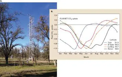
uptake (the negative values on the y -axis) for forests at four different latitudes. It shows that the higher the latitude of the forest, the later in summer its CO 2 uptake peaks. Such measurements provide the basis for modeling global climate change and for negotiating agreements to “trade” pollution for forest growth. Note, however, that being a greenhouse gas does not make CO 2 inherently “bad” for the environment. In fact, if heterotrophic production of CO 2 were to cease altogether, phototrophs would run out of CO 2 in roughly 300 years, despite the vast quantities of carbon present in the ocean and crust. Thus, both CO 2 fixers and heterotrophs need each other for a continuous cycle.
Carbon Cycling by Different Ecosystems
Different kinds of ecosystems, such as marine and terrestrial ecosystems, cycle carbon in different ways. Access to oxygen is a major factor in determining the rate of carbon cycling and the form of carbon stored in sinks.
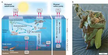
Marine carbon cycling. The largest aerated ecosystem is the photic zone of oceans (Fig. 22.4A). In the aerated (or oxic) habitat of the marine photic zone, the ecosystem absorbs enough light for the rate of photosynthesis to exceed the rate of heterotrophy. Photosynthesis drives what is called the biological carbon pump. Microbial and plant photosynthesis fixes CO 2 into biomass, designated by the shorthand [CH 2 O]. Photoautotrophs that fix carbon include bacteria and protists. Marine phototrophs such as diatoms and coccolithophores trap a substantial amount of carbon in biomass (Fig. 22.4B ). A portion of their biomass sinks to the ocean floor through the weight of their silicate or carbonate exoskeletons. FIGURE 22.4 ■ The ocean’s biological carbon pump. A. In the biological carbon pump, CO 2 is fixed by phytoplankton. Aerobic respiration by zooplankton and mixotrophs converts some biomass back to CO 2, while other biomass sinks to the deep ocean. In the physical carbon pump (at right), atmospheric CO 2 dissolves in the ocean and enters equilibrium with carbonates, releasing H + ions. The CO removal decreases the greenhouse
2
effect, but as H + is released the ocean acidifies. B. Diatoms in lake sediment store carbon (colorized SEM).
EYE OF SCIENCE/SCIENCE SOURCE
Photosynthetic CO 2 fixation is accompanied by release of O 2. The O 2 is then used by heterotrophs (such as bacteria, protists, and animals) to convert [CH 2 O] back to CO 2. In the presence of light, a net excess of O 2 is released. Biomass is also produced through lithotrophy or chemolithoautotrophy—the oxidation of hydrogen, hydrogen sulfide, ferrous iron (Fe 2+) and other reduced minerals, and even carbon monoxide.
Marine methanogenesis. At the benthos, marine microbial metabolism generates a redox gradient from oxic to anoxic (discussed in Chapter 14). The anoxic region supports methanogenic
archaea (methanogens, discussed in Chapter 19). The methane released forms methane hydrates. Warming of methane hydrates may lead to release of gaseous methane, which in turn amplifies the greenhouse effect that warms the planet, in a positive feedback loop. Although methane represents a relatively small fraction of the atmosphere (CO 2 levels are 200-fold higher than methane levels), it traps 80-fold more heat within 20 years after release.
An important part of global climate calculations is accounting for the rate of methane production by methanogens, such as Methanosaeta and Methanosarcina.
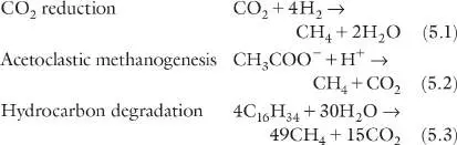
The modes of methane output turn out to be surprisingly complex. Some examples include: The simplest form of methanogenesis involves H 2 reduction of CO 2 (Equation 5.1), both of which are products of bacterial fermentation. But methanogens can also convert other bacterial fermentation products such as acetate (Equation 5.2). Even petroleum can be converted directly to methane (Equation 5.3), as shown in 2021 by Zhuo Zhou and colleagues at the Biogas Institute, Chengdu, China. Zhou’s group isolated candidate species “ Candidatus Methanoliparia” from an enrichment culture using oily sludge from a subsurface petroleum reservoir. Methane production from oil (Equation 5.3) was demonstrated by 13 C-labeling of hexadecane (C H). After 100
16 34
days incubation, “ Ca. Methanoliparia” converted most of the substrate to 13 C-labeled methane. This reaction represents another
large factor that scientists must consider in our calculations predicting global warming.
Another source of marine methane is the aerobic ammonia-oxidizing archaea, such as Nitrosopumilus (discussed in Chapter 19). William W. Metcalf and colleagues at the University of Illinois at Urbana-Champaign showed that Nitrosopumilus species conduct reactions that degrade phosphonates, organic compounds containing a direct carbon-phosphorus bond. The reactions release methylphosphonate, a compound that many kinds of bacteria convert to methane in order to acquire the scarce phosphate for phospholipids and nucleic acids. Many bacteria, as well as archaea, release methane from methylphosphonate in the aerated water column.
Methane oxidation. Certain bacteria and archaea oxidize methane to carbonates or CO 2, thus limiting the rise of atmospheric methane. Methane-oxidizing bacteria are ubiquitous in all environments of water and soil. Examples include many Gammaproteobacteria, Alphaproteobacteria and Verrucomicrobia. Methane is also removed by anaerobic methane-oxidizing archaea (ANME) such as Methanoperedenaceae. At the ocean floor, some of the methane hydrates are oxidized by microbial mats of sulfate-reducing bacteria and anaerobic methane-oxidizing archaea (ANME), discussed in Section 19.4. The sulfate reducers plus the methane oxidizers conduct a syntrophic reaction, for which the overall Δ G value is negative: CH + SO 2− → HCO − + HS − + H O
4 4 3 2
In this metabolism, methane is the initial electron donor oxidized by the ANME partner, and sulfate is the terminal electron acceptor reduced by the bacteria. The high sulfate concentration of marine water drives this reaction in anoxic sediment, where all of the O 2 has been consumed by microbes that oxidize upwelling reduced minerals (such as sulfide oxidizers at thermal vents and cold seeps, discussed in Chapter 21).
Terrestrial carbon cycling. Another large aerobic habitat is the oxygenated layer of soil (discussed in Chapter 21; Fig. 22.5A, top). While plants perform most of the terrestrial photosynthesis, microbial phototrophs found in soil also fix CO 2 into biomass. Microbial lithotrophy fixes carbon in soil and in weathered areas of crustal rock. Lithotrophy is performed solely by bacteria and archaea, essential microbial partners in these ecosystems. Unlike photosynthesis, lithotrophy usually consumes O 2 instead of producing it. Much carbon is stored as carbon polymers such as cellulose and lignin. But microbial and animal consumers release a lot of CO 2 through respiration.
FIGURE 22.5 ■ The terrestrial carbon cycle: aerobic and anaerobic. A. Aerobic and anaerobic conversions of carbon. Blue = reduction of carbon; red = oxidation of carbon; orange = fermentation; [CH 2 O] = organic biomass. In an aerobic environment (top), photosynthesis generates molecular oxygen (O 2), which enables the most efficient metabolism by heterotrophs, methanotrophs, and lithotrophs. B. Cortinarius armillatus mushrooms are fruiting bodies of mycorrhizal fungi that
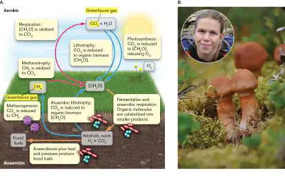
share mutualism with birch trees. Inset: Karina Clemmensen studies mycorrhizal sequestration of carbon.
©ÓKASPER ANDERSON
COURTESY OF KARINA CLEMMENSEN
In 2013, another important microbial carbon sink was discovered by Karina Clemmensen, Björn Lindahl, and colleagues at Uppsala BioCenter, Sweden: the mycorrhizal fungi (presented in Chapter 21). Mycorrhizal fungi (Fig. 22.5B ) form mutualistic associations with forest plant roots and are especially important for the roots of trees. Clemmensen showed that in some forests, the roots and fungi can sequester as much as 22 kilograms of carbon per square meter of forest soil, which may be 70% of the total carbon sequestered. Thus, mycorrhizal fungi play an important role in minimizing release of the greenhouse gas CO 2.
Beneath the aerated soil, microbial metabolism generates a steep redox gradient down into anoxic layers (discussed in Chapters 14 and 21). Anoxic regions support lower rates of biomass production than do oxygen-rich environments because they depend on oxidants of lower redox potential and limited quantity, such as Fe 3+. Anaerobic conversion of CO 2 to biomass is done mainly by bacteria and archaea. Vast, permanently anaerobic habitats extend several kilometers below Earth’s surface, encompassing a greater volume than the rest of the biosphere put together (Fig. 22.5A, bottom). In these habitats, endolithic bacteria inhabit the interstices of rock crystals (discussed in Chapter 21).
In soil and water, anaerobic metabolism includes fermentation of organic carbon sources, as well as respiration and lithotrophy with alternative electron acceptors such as nitrate, ferric iron (Fe 3+), and sulfate. Anaerobic decomposition by microbes is one stage in the formation of fossil fuels such as oil and natural gas (primarily methane). In soil, anoxic conditions (extremely low levels of O 2) favor incomplete catabolism. Recall from Chapter 13 that glycans are broken down to sugars, which undergo glycolysis to pyruvate. Without oxygen, pyruvate is rearranged via fermentation to products such as lactate, ethanol, and acetate, as well as the gases CO 2 and H 2. The partly decomposed matter becomes available for further decomposition when terminal electron acceptors appear. But anoxic environments also favor production of methanogenesis (discussed in Chapters 14 and 19).
The Global Carbon Balance and Temperature Change
How do we know that our climate is changing? It is difficult for us to tell from one year to the next, but historical records show that since the beginning of the industrial age, atmospheric CO 2 has risen steeply (Fig. 22.1A). The rise of CO 2 is supported by several forms of evidence, most notably the measurement of CO 2 concentrations in ice cores drilled from polar glaciers. Results of climate modeling are consistent with the greenhouse effect causing our global rise of temperature by 1°C since 1800. Another half-degree increase is likely within the next decades, and there’s no sign of stopping. A total increase of 2°C will likely eradicate corals and make many population centers uninhabitable because of extreme heat.
Through their release of CO 2, organotrophic organisms (including microbes, as well as multicellular eukaryotes) are at present the major agent of global temperature rise. The rise in temperature results from radiative forcing (Fig. 22.6). Radiative forcing is defined as the difference between the sunlight energy absorbed by Earth and the energy radiated out to space. Forcing is measured in units of solar radiation energy over time (watts) absorbed per square meter of the planet’s surface. Some solar radiation is reflected back to space by light-colored surfaces such as clouds and snow, known as the “albedo” effect.
FIGURE 22.6 ■ Sources of radiative forcing that lead to global warming. Radiative forcing is the increase in warming of Earth’s atmosphere (in watts per square meter) associated with a particular climate factor. The total radiative forcing ascribed to human activity (anthropogenic) is calculated at 1.6 watts per square meter (W/m 2).
Source: Modified from Intergovernmental Panel on Climate Change. 2007. Climate Change 2007. Cambridge University Press, fig. SPM.2.
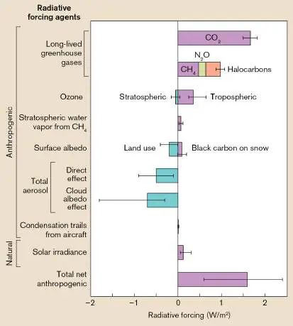
Climate scientists combine many sources of data to generate computed models of how the climate is changing, and which factors have the greatest effect. Besides CO 2, important agents of radiative forcing include methane (CH 4) and nitrous oxide (N 2 O); the latter is discussed in Section 22.3.
The level of atmospheric CO 2 depends largely on the global balance of biological CO 2 fixation and release by combustion and catabolism. A major part of the recent increase comes from the combustion of fossil fuels, which adds about 6 × 10 15 grams of carbon annually to the atmosphere. Fossil fuels are the product of microbial anaerobic digestion of plant and animal remains, reduced to hydrocarbons by the pressure and heat of Earth’s crust. When burned as fuel, carbon that had accumulated over millions of years is rapidly returned to the atmosphere as CO 2. Increased CO 2 fixation and ocean absorption compensate for some of the CO 2 flux, but about a tenth of the carbon remains in the atmosphere.
Another major factor in CO 2 flux is land use for beef production. Cattle and their gut microbes are a major source of CO 2. Substantial carbon reductions could occur if consumers switch from beef burgers to plant products engineered for beef taste, such as the Impossible Burger (presented in Chapter 18).
The rise of CO 2 in our atmosphere is limited by abiotic factors. Most important, oceans dissolve more than half of the CO 2 entering Earth’s atmosphere. But the dissolved CO 2 reacts to form carbonic acid, which releases hydrogen ions and thus lowers the pH: CO + H O ⇌ H CO ⇌ HCO − + H + ⇌ CO 2− + 2H +
2 2 2 3 3 3
Ocean acidification is harmful to corals and zooplankton that have shells of calcium carbonate, which dissolves with acid.
Arctic methanogens accelerate global warming. A major agent of radiative forcing is atmospheric methane (Fig. 22.6). Methane is a relatively small component of the atmosphere (0.00019%), but its radiative forcing factor is 25 times that of CO 2. Methane release is increasing at exceptional rates, especially in the Arctic tundra. Geological evidence suggests that rapid methane release accompanied the retreat of the glaciers during ice age transitions. Today, as Arctic tundra melts, we again see rapid rise of methane as exemplified by combustible release from Arctic lakes (Fig. 22.7). A common methanogen in the tundra is Methanosarcina species.
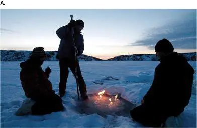
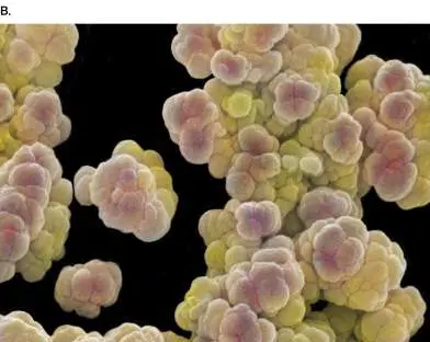
FIGURE 22.7 ■ Methane from methanogens in Arctic lakes. A. Researchers ignite a bubble of methane on Alaska’s Seward Peninsula. B. Methanosarcina sp., a type of methanogen whose metabolism is accelerated by global warming.
LUIS SINCO/LOS ANGELES TIMES VIA GETTY IMAGES
POWER AND SYRED/SCIENCE SOURCE
How can we assess the climate threat of methane release from thawing tundra? The Arctic tundra is estimated to store more than twice the amount of carbon than exists in the atmosphere. Large quantities of dead plant matter are stored in permanently frozen soil, called permafrost. But today the permafrost is thawing. As permafrost thaws, it accelerates microbial decomposition of material that was accumulated over tens of thousands of years (Fig. 22.8A).
Bacterial fermentation products include CO 2 and acetate, which methanogens reduce to methane. The acceleration of methane
release is amplified by a positive feedback loop (Fig. 22.8B ). As CH 4 emerges from the soil and enters the atmosphere, its radiative forcing (greenhouse effect) increases temperature, which further accelerates the thawing of permafrost.
FIGURE 22.8 ■ Thawing permafrost accelerates methane release by methanogenic archaea. A. Stordalen Mire, Sweden, a model site for study of thawing permafrost. B.
Atmospheric CH 4 raises global temperature, which then accelerates thawing and methane release by methanogens, in a positive feedback cycle. C. Palsa, with permafrost; bog, with soil partly melted; fen, fully melted and anoxic. D. Eun-Hae Kim, a student of Virginia Rich, collects samples from Stordalen Mire. E. Phylogeny of metagenome-assembled genomes (MAGs) of methanogenic archaea identified from Stordalen bogs and fens.
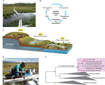
The scale is based on the mean number of substitutions per nucleotide.
Sources: Parts C and E modified from Ben Woodcroft et al. 2018. Nature 560
:49–54, fig. 1 (C) and extended data fig. 1 (E).
COURTESY OF CARMODY MCCALLEY
COURTESY OF VIRGINIA RICH
Virginia Rich at the Ohio State University and Scott Saleska at the University of Arizona study the process of thawing permafrost and the resulting succession of microbial communities. Their study at Stordalen Mire, in Sweden, addresses questions such as: Which microbes decompose thawed organic matter? Which species form methane? And which species consume methane before it enters the atmosphere?
Stordalen Mire is a model site for thawing permafrost because it includes examples of three stages (Fig. 22.8C ): Palsa—the soil above solid permafrost Bog—permafrost that is partly thawed, with some frozen underneath Fen—fully thawed, anoxic wetland At Stordalen Mire, Rich’s students collect samples of tundra at different stages of thawing, including palsa, bog, and fen (Fig. 22.8D ). From the samples, the students sequence DNA and obtain metagenome-assembled genomes (MAGs) by procedures described in Chapter 21. Thawing permafrost yields diverse communities of bacteria and archaea, with key species predominating in each of the three stages. Methanogenic archaea (Fig. 22.8E ) are most abundant in the anoxic fen, including candidate species such as Methanoflorens stordalenmirensis, which are unique to the Stordalen site.
By sampling all three thawing stages, Rich has mapped a picture of the overall microbial community succession (shift in predominant taxa, a concept discussed in Chapter 21). The three tundra types— palsa, bog, and fen—are color-coded orange, green, and light purple, respectively, throughout Figure 22.9. For each metabolic process, such as cellulose degradation or xylan degradation, color-coded box plots show the relative abundance of metagenome-assembled genomes (MAGs) that encode enzymes for the respective pathway. The bubble plots indicate the relative abundance of MAG taxa (coded in the clade list of Fig. 22.9).
FIGURE 22.9 ■ Decomposition, methanogenesis, and methanotrophy in microbial communities of thawing permafrost (palsa, bog, and fen). Box plots show relative abundance of MAGs that encode the pathway indicated. Bubble
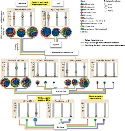
plots contain circles colored by phylum; circle size represents the relative abundance of each MAG.
Source: Modified from Ben Woodcroft et al. 2018. Nature 560 :49–54, fig. 2. For plant matter breakdown and fermentation, MAGs appear in all three stages of thawing. But the fens (fully thawed) show the highest levels of methanogenesis, both by CO 2 reduction and by acetate reduction (that is, they are acetoclastic). Most interesting, in the fens Rich found MAGs of methanotrophs, methane-oxidizing bacteria. These bacteria oxidize methane to yield energy and fix carbon into biomass when molecular oxygen is available. Calculations show that methanotrophs consume a substantial portion of methane before it reaches the air. Thus, understanding the methanotrophic bacteria (see Chapter 14) may help us find ways to mitigate the Arctic release of methane.
Human attempts to alter or mitigate global temperature rise. Could human technology provide a fix to climate change? Some human-associated factors can decrease radiative forcing, such as the production of sulfate aerosols (suspended particles or droplets) in the upper atmosphere. Measurements of these factors have led some scientists to propose controversial experiments to reverse or prevent global warming. For example, in 2022, scientists at the Massachusetts Institute of Technology proposed constructing a giant shield of silicon bubbles in space to deflect enough solar radiation to decrease global warming. However, the proposed project requires technologies not yet invented, and even a successful implementation would not remove the need to replace burnable fuels with sustainable energy. The unpredictable effects of these global experiments have discouraged such attempts.
From a political standpoint, ecosystems such as forests that act as carbon sinks by fixing carbon into stable biomass are considered desirable because they lessen the rate of CO 2 input into the atmosphere. The question is complex because CO 2 -generating ecosystems provide other environmental benefits. For example, wetlands are among Earth’s most productive ecosystems, supporting vast amounts of plant and animal life, although they also release significant amounts of CO 2 and methane.
To Summarize
Microbes cycle essential elements in the biosphere.
Many key cycling reactions are performed only by bacteria and archaea. Methanogenic archaea (methanogens) produce methane, a potent greenhouse gas.
Elements cycle between organisms and abiotic sources and sinks. The most accessible source of carbon and nitrogen is the atmosphere. Earth’s crust stores large amounts of key elements, but their availability to organisms is limited. Carbon cycling involves changes in oxidation state. The more oxidized forms of carbon are found near Earth’s surface or in the atmosphere, whereas the more reduced forms accumulate deep underground. Atmospheric carbon cycles are severely perturbed by the burning of fossil fuels.
Environmental flux of elements is measured through chemistry. Methods include infrared spectroscopy and mass spectrometry, gas chromatography, radioisotope incorporation, and the measurement of stable isotope ratios.
Cyanobacteria and other phytoplankton consume much of the biospheric CO 2 and release O 2. Oxygen released by phototrophs is used by aerobic heterotrophs and lithotrophs. Marine plankton, as well as terrestrial trees and mycorrhizal fungi, serve as major carbon sinks.
Anaerobic environments cycle carbon through bacteria and archaea. Bacteria conduct fermentation and anaerobic respiration, while methanogens convert CO 2 and H 2 to methane. Methane is oxidized to CO 2 by methane-oxidizing bacteria and archaea.
Radiative forcing is the increase of global warming associated with a particular chemical agent. At present, the major source of radiative forcing is the net rise of atmospheric CO 2. Microbial decomposition returns CO 2 and CH 4 to the atmosphere and accelerates global warming. Thawing of Arctic permafrost is a growing source of radiative forcing. Permafrost thawing activates microbes to convert tens of thousands of years’ accumulation of organic matter to CO 2 and methane.
Glossary
abiotic Produced without living organisms; occurring in the absence of life.
biotic Caused by living organisms.
biogeochemical cycle The recycling of elements needed for life (such as carbon or nitrogen) through the biotic and abiotic components of the biosphere.
biogeochemistry Also called geomicrobiology. The metabolic interactions of microbial communities with the abiotic (mineral) components of their ecosystems.
geomicrobiology See biogeochemistry .
greenhouse effect The trapping of solar radiation heat in the atmosphere by CO 2; a cause of global warming.
reservoir 1. The major part of the biosphere that contains a significant amount of an element needed for life. 2. An organism that maintains a virus or bacterial pathogen in an area by serving as a high-titer host.
source A part of the biosphere that stores a significant quantity of a given element; may be biotic (as in tree biomass, a source of carbon) or abiotic (as in carbonate rock).
sink A part of the biosphere that can receive or assimilate significant quantities of an element; may be biotic (as in plants fixing carbon) or abiotic (as in the ocean absorbing carbon dioxide). mesocosm A small, controlled model ecosystem.
biological carbon pump The fixation of carbon dioxide by phototrophs and gravitational settling of biomass particles within the oceans.
radiative forcing The increase in warming of Earth’s atmosphere (in watts per square meter) associated with a particular climate factor, which is calculated as the difference between the sunlight energy absorbed by Earth and the energy radiated out to space. fossil fuel Ancient organismal remains that have been converted to hydrocarbons (petroleum and natural gas) or sedimentary rock (coal) through microbial digestion followed by reduction under high pressure underground. Fossil fuels are extracted and burned by humans for energy.
22.2 The Hydrologic Cycle and Wastewater Treatmentnot assigned
The distribution of complex carbon compounds is largely a function of the hydrologic cycle, or water cycle, the cyclic exchange of water between atmospheric water vapor and Earth’s ecosystems (Fig. 22.10A). In the hydrologic cycle, water precipitates as rain, which is drawn by gravity into groundwater, rivers, lakes, and ultimately the ocean. The ocean supplies a vast reservoir of water. All along the cycle, evaporation returns water to the air. Human communities interact with the hydrologic cycle by drawing water for drinking and other purposes, and by returning wastewater. Before wastewater can be safely returned to the hydrologic cycle, organic contaminants must be removed. Key parts of that treatment are performed by microbes.
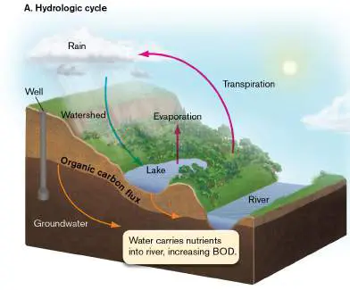
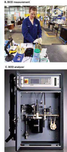
FIGURE 22.10 ■ The hydrologic cycle interacts with the carbon cycle. A. The hydrologic cycle carries bacteria and organic carbon into groundwater and aquatic systems. B. Bottled water samples are measured for dissolved oxygen over time; the rate of decrease of dissolved oxygen indicates biochemical oxygen demand (BOD). The rate of decrease of dissolved oxygen in water samples is approximately proportional to the concentration of organic matter available for respiration. C. A microprocessor-controlled BIOX-1010 BOD analyzer measures rate of respiration. Water samples are mixed with a concentrated microbial biomass, and a dissolved-oxygen (DO) sensor measures small rates of oxygen decrease over time.
AP PHOTO/THE CASPER STAR–TRIBUNE, ALAN ROGERS
ENVITECH LTD.
Biochemical Oxygen Demand
What determines the health of an aquatic ecosystem? As discussed in Chapter 21, a major factor in the health of ecosystems is the balance between the level of oxygen and the levels of reduced organic nutrients. Organic contamination destabilizes marine, freshwater, and terrestrial ecosystems. Water passing through soil and aquatic ecosystems carries organic carbon material from humus, sewage, and fertilizer runoff. A sudden influx of rich carbon substrates accelerates respiration by aquatic microbes. Microbial respiration then competes with respiration by fish, invertebrates, and amphibians for the limited supply of oxygen dissolved in water, raising the biochemical oxygen demand (BOD), also called the biological oxygen demand. The higher the concentration of organic substances, the higher the BOD arising from microbial oxygen consumption.
High BOD can cause massive die-off of fish and other aquatic animals. Thus, a routine part of monitoring the health of lakes and streams is the measurement of BOD from water samples (Fig.
22.10B ). Oxygen uptake is observed in a BOD analyzer (Fig.
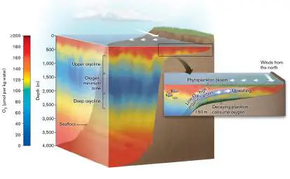
22.10C ), which detects dissolved oxygen in water. The rate of decrease of dissolved oxygen measured by the BOD analyzer is approximately proportional to the amount of dissolved organic matter available for respiration. Note, however, that the BOD in a natural environment will depend on the microbes actually present, as well as the plants and animals competing for oxygen and other resources. In the past, BOD was considered a local issue, affecting the health of lakes and rivers in a community. But today we recognize huge effects of rising BOD in the oceans (Fig. 22.11). Ocean oxygen levels are high near the surface, where phototrophs release oxygen, but organic nutrients are so scarce that respiration is limited. Oxygen is also concentrated in the deep benthos, because most organic nutrients have been consumed, and because the sheer volume of water can hold dissolved oxygen in large amounts. But near the coastal shelf, currents may carry sediment up to a middle region where organic nutrients meet the oxygen. This combination supports rapid bacterial respiration. The result is an oxygen minimum zone (OMZ), a region of low or near-zero oxygen sandwiched between the upper and lower oxygenated layers. Oxygen minimum zones support anaerobic microbial communities but cannot support fish and invertebrate animals. Above and below the anoxic water, there is a steep oxycline (gradient of oxygen concentration) to the upper and lower regions where oxygen is available. A well-known OMZ is located off the coast of Oregon, where crabs and other animals are found dying as they try to escape asphyxiation.
FIGURE 22.11 ■ Oxygen minimum zone in the ocean. The oxygen minimum zone (OMZ) occurs in the region of the coastal shelf where nutrients from below meet the oxygen produced by phototrophs above. In this region, microbial respiration consumes oxygen faster than it is replenished. Below, organic nutrients are too dilute for much oxidation, and O 2 remains available. The OMZ can expand upward when phytoplankton blooms decay, consuming the surface oxygen.
Oxygen minimum zones are worsened by increasing temperatures, which accelerate respiration, and by influx of sewage and agricultural waste. The zone expands upward toward the surface and downward to the sediment, trapping crabs and fish. Today, large regions of ocean have become dead zones, or zones of hypoxia, devoid of most fish and invertebrates. A major dead zone is a region in the Gulf of Mexico off the coast of Louisiana where the Mississippi River releases about 40% of the U.S. drainage into the sea (Fig. 22.12A). Over its long, meandering course, which includes inputs from the Ohio and Missouri rivers, the Mississippi builds up high levels of organic pollutants, as well as nitrates from agricultural fertilizer. When these nitrogen-rich substances flow rapidly out to the Gulf of
Mexico in the spring, they lift the nitrogen limitation on algal growth and feed massive algal blooms. The algal population then crashes, and its sedimenting cells are consumed by heterotrophic bacteria. The heterotrophs use up the available oxygen, causing hypoxia. Hypoxia kills off the fish, shellfish, and crustaceans over a region equivalent in size to the state of New Jersey.
FIGURE 22.12 ■ The dead zone in the Gulf of Mexico. A. The Mississippi River drainage (shaded green) empties into the Gulf of Mexico. Every summer, drainage high in organic carbon and nitrogen causes algal blooms, leading to hypoxia and death of fish. B. Aerial view of the oil leaked from the Deepwater Horizon oil wellhead in the Gulf of Mexico in 2010.
Source: Part A based on data from the National Oceanographic and
Atmospheric Administration.
AP PHOTO/ERIC GAY
In 2010, the Gulf of Mexico dead zone was expanded by the unprecedented spill of oil from the Deepwater Horizon oil well blowout (Fig. 22.12B ; discussed in Chapter 21). Many
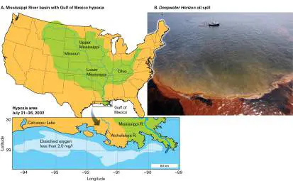
of the pollutants were metabolized to CO 2 by oil-eating bacteria that feed naturally on oil seeping slowly from Gulf of Mexico sediment. But the sudden large input of oil raised microbial respiration and BOD levels throughout the Gulf of Mexico, thus lowering the amount of oxygen available to wildlife. Dead zones now occur along the coasts of industrial and developing countries throughout the world, including Australia and India. Dead zones deplete habitat for much marine life; for example, forcing sharks to swim out of hypoxic regions and nearer the shore. Dead zones contribute to the crash of fisheries worldwide, removing a critical food resource for human populations. To avoid such dead zones, release of industrial pollutants and fertilizers must be prevented. In addition, all the communities throughout the river drainage areas must treat their wastes to eliminate nitrogenous wastes before disposal.
There are two common approaches to community wastewater treatment, both of which involve microbial partners: wastewater treatment plants and wetland filtration. Both approaches depend on microbes to remove organic carbon and nitrogen from water before it returns to aquatic systems and ultimately the ocean.
Wastewater Treatment in Our Built Environment
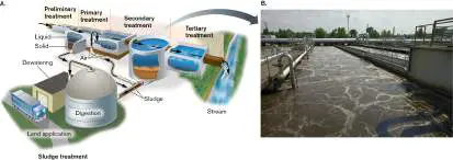
In industrialized nations, we supply our “built environment” with clean water, free of toxicants and pathogens. Most municipal communities use some form of wastewater treatment (Fig. 22.13). The human sewage component of wastewater contains liquid and solid wastes produced by the human digestive and excretory systems. The purpose of wastewater treatment is to decrease the BOD and the level of human pathogens before water is returned to local rivers. The treatment process includes microbial metabolism. The process requires a highly sophisticated facility with complex engineering to maximize the efficiency of microbial catabolism. A wastewater treatment plant can convert sewage into water that exceeds all government standards for humans to drink.
FIGURE 22.13 ■ Wastewater treatment with bioremediation. A. In a municipal treatment plant, wastewater undergoes primary treatment (filtering and settling), secondary treatment (bioremediation by microbial decomposition), and tertiary treatment (chemical treatments including chlorination and dechlorination). B. Aeration basin for secondary treatment with microbes.
DESINTEGRATOR/ALAMY STOCK PHOTO
The wastewater treatment plant is the final destination for all household and industrial liquid wastes passing through the municipal sewage system. A typical plant includes the following stages of treatment, illustrated in Fig. 22.13A.
Preliminary and primary treatment. Preliminary treatment consists of screens that remove solid debris, such as sticks, dead animals, and personal hygiene items. Primary treatment includes fine screens and sedimentation tanks that remove insoluble particles. The particles eventually are recombined with the solid products of wastewater treatment to form what is known as sludge. The sludge ultimately is used for fertilizer or landfill.
Secondary treatment. Secondary treatment consists primarily of microbial ecosystems that decompose the soluble organic content of wastewater by aerobic and anaerobic respiration. The nutrient removal process may include biological removal of nitrogen and phosphorus: Nitrogen is removed by nitrifying bacteria that oxidize
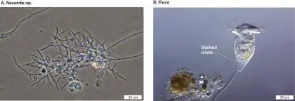
ammonium, and phosphorus is removed by polyphosphate-accumulating bacteria. The microbes form particulate flocs of biofilm. Floc microbes typically include bacilli such as Zoogloea, Flavobacterium, and Pseudomonas, as well as filamentous species such as Nocardia (Fig. 22.14A). A multilevel ecosystem forms, in which the bacteria are preyed on by protists such as stalked ciliates ( Fig. 22.14B ), swimming ciliates, and amebas, as well as invertebrates such as rotifers and nematodes. The predators serve the valuable function of limiting the numbers of planktonic single-celled bacteria, enabling the bulk of the biomass to be removed by sedimentation.
FIGURE 22.14 ■ Microbes in wastewater bioremediation. A. Secondary treatment generates flocs held together by filamentous bacteria, commonly Nocardia sp. (LM). B. Stalked ciliates in flocs prey on bacteria (LM).
WENDA HOWARD, VIREO ENVIRONMENTAL LLC
FRANK FOX/SCIENCE SOURCE
The microbial ecosystems of secondary treatment require continual aeration to maximize the breakdown of molecules to carbon dioxide and nitrates. The floc size and composition must be monitored for optimal performance. Optimal treatment depends on the ratio of filamentous to single-celled bacteria: enough filaments to hold together the flocs for sedimentation, but not so many as to trap air and cause flocs to float and foam, preventing sedimentation. As
the flocs build up, they are sedimented as sludge and are known as activated sludge, owing to their microbial activity.
The ecosystem of activated sludge includes filamentous methanogens (discussed in Chapter 19), which metabolize short-chain molecules such as acetate within the anaerobic interior of flocs. Thus, wastewater treatment generates methane, often in quantities that can be recovered as fuel.
Wastewater Monitoring of Pathogens. The wastewater influent (upstream of any treatment) contains a wide range of pathogens excreted by the human and animal community. Human bacterial pathogens commonly include enteric bacteria such as Salmonella, Shigella, and Escherichia species. Common protozoan pathogens include Giardia lamblia and Cryptosporidium. Important viral pathogens include noroviruses, sapoviruses, and enteroviruses such as poliovirus. Noroviruses and sapoviruses are major causes of acute viral gastroenteritis (intestinal inflammation; see Chapter 26). Enteroviruses are highly prevalent in wastewater and may cause a flu-like illness with occasional symptoms resembling polio. The removal of such viruses is a growing concern, as human populations enlarge and concentrate around shared water sources.
The pathogen content of wastewater offers a public health opportunity for community surveillance of the prevalence of serious illnesses. In 2022, wastewater surveillance detected poliovirus in several counties of New York State. (Poliovirus replication and transmission are described in eAppendix 4.) Finding poliovirus came as a surprise, as the United States and many other countries were considered free of polio since the 1990s, with the rare exception of occasional travelers from polio-endemic regions. Yet in 2022 New York saw one local case of poliomyelitis (paralytic polio), and wastewater surveillance tracked community spread of the virus through several counties. The wastewater detection was particularly important because most individuals are unaware of infection yet can transmit the virus to someone who develops paralysis. Transmission and illness are completely preventable by polio vaccine.
The detection of virus in wastewater is accomplished by quantitative RT-PCR (reverse-transcriptase polymerase chain reaction) a method in which reverse-transcribed viral RNA generates DNA copies that are amplified by PCR (a method shown in Chapter 6, Figure 6.30). This remarkable technique can detect single molecules of viral RNA in a sample. The method first came into widespread use during the COVID-19 pandemic, when wastewater was monitored effectively for the coronavirus SARS-CoV-2. For this virus, actual virions do not survive in the wastewater, but viral RNA molecules are surprisingly persistent. The viral RNA concentrations from a given community could be detected and quantified by digital RT-PCR (Fig. 22.15A). Typically, the wastewater virus signal rises a week before case reports appear, giving the local health infrastructure some warning ahead. A signal that appears ahead of a trend is called a leading indicator. In the case of the coronavirus, viral RNA continues to be shed after patients have recovered from symptoms, so it also becomes a “lagging indicator” of community recovery.
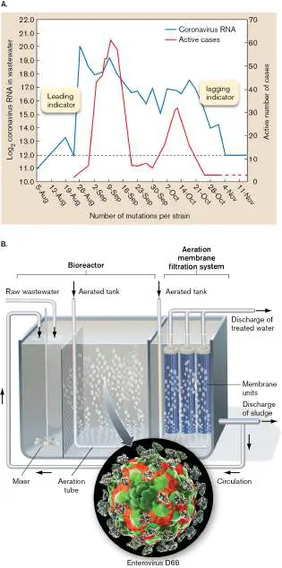
FIGURE 22.15 ■ Viruses in wastewater. A. Wastewater monitoring detects SARS-CoV-2 viral RNA (not live virus) in untreated wastewater by use of digital RT-PCR. Viral RNA appears before community COVID-19 case reports rise. B. During secondary treatment, membrane bioreactor filtration removes sludge particles and enteric viruses. Inset: Enterovirus D68; model based on cryo-electron microscopy.
KATERYNA KON/SCIENCE SOURCE
Ideally, all pathogens would be removed by wastewater treatment. Biological and chemical treatment can be highly effective at removing bacterial pathogens such as Salmonella or Vibrio cholerae. It is less effective at removing viral pathogens such as enteroviruses that survive higher levels of chlorination. Viruses and other human pathogens are most effectively removed by membrane bioreactors (Fig. 22.15B ). The bioreactor consists of hollow-fiber membranes submerged in the biologically active floc suspension during secondary treatment. The influent undergoes microfiltration (pore size 0.1–0.4 μm) or ultrafiltration (0.01–0.04 μm). These pore sizes are not small enough for the complete removal of enteroviruses, which are typically 0.03 μm in size. Nevertheless, the pores exclude floc particles to which the viruses adhere, and they greatly decrease the virus titer in the effluent. Note that disposal of the virus-contaminated sludge requires further disinfection.
Tertiary (advanced) treatment. Tertiary treatment (see diagram, Fig. 22.13A) includes filtration of particulates from the microbial flocs of secondary treatment, and it may include chemical processes to decrease nitrogen and phosphorus. The final step involves disinfection to eliminate pathogens, usually by a chemical process such as chlorination; that is, treatment with hypochlorite ion (ClO −). The water must then undergo dechlorination, commonly with sulfur dioxide, to convert remaining hypochlorite to chloride ion (Cl −) and avoid formation of chlorinated organic toxicants.
Following the full wastewater treatment cycle, the treated water is then returned to local streams and lakes. Few people realize that their familiar freshwater sources are receptacles for microbiologically treated wastewater.
Thought Question
22.2 What would happen if wastewater treatment lacked microbial predators? Why would the result be harmful?
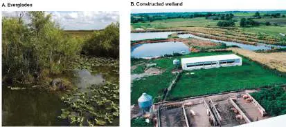
Agricultural treatment. Wastewater treatment plants are impractical for purifying the runoff from large agricultural operations. For large-scale alternatives to treatment plants, communities and agricultural operations are looking to wetland restoration. Much of our current water supply is already filtered and purified by natural wetlands, such as the Florida Everglades (Fig. 22.16A). Wetlands remove nitrogen through the action of denitrifying bacteria. In wetlands, rainwater and river water trickle slowly through vast stretches of soil, where microbial conversion acts as the foundation of a macroscopic ecosystem that includes trees and vertebrates. Thus, much of the carbon and nitrogen is fixed into valuable biomass. In the wetlands of the Everglades, the remaining water filters slowly through limestone into underground aquifers, which ultimately provide water through wells to human communities.
FIGURE 22.16 ■ Water filtration by wetlands. A. The marshes of the Everglades act as natural filters that bioremediate water entering the aquifers of southern Florida. B. The filtering system that Steve Kerns installed on his hog farm in Taylor County, Iowa, consists of a series of hillside terraces that form constructed wetlands. The constructed wetlands contain microbial communities that metabolize hog manure and wastewater.
JOAN SLONCZEWSKI
TIM MCCABE/USDA/NRCS
Some agricultural operations are building artificial wetlands, known as constructed wetlands, to replace treatment plants. A constructed wetland is a built environment designed to provide environmental services comparable to those of natural wetlands. Figure 22.16B shows a hog farm where a series of terraced wetlands was built to drain liquefied manure. The wetlands were found to produce fewer odors and to remove organics more efficiently and at a lower cost than do traditional filtration plants.
A much greater challenge is that of industrial runoff, in which toxic wastes from factory chemistry enter an aquifer at levels endangering human health. These chemicals may poison the treatment plants designed for human effluents. Large regions of land surrounding such a plant may require remediation that is expensive or impractical. And traces of pollutants such as chlorinated aromatics reach every spot on
the globe; for example, dioxins are found in the tissues of Antarctic penguins.
How can we remediate industrial pollutants before they poison the local countryside and spread throughout the globe? One way is to harness naturally occurring bacteria for bioremediation. The bacterial community’s reaction rate can be enhanced through selection by enrichment culture (described in Chapter 21). In the culture, organisms from the polluted site are cultivated repeatedly in the presence of added pollutant, and then tested for activity using radiolabeled substrates. For example, microbial communities obtained from marine plastic detritus can be cultured to isolate plastic-eating bacteria.
To Summarize
The hydrologic cycle is the cyclic exchange of water between the atmosphere and the biosphere. Water precipitates as rain, which enters the ground and ultimately flows to the oceans. Along the way, some of the water evaporates, returning to the atmosphere.
Water carries organic carbon that generates biochemical oxygen demand (BOD). High BOD accelerates heterotrophic respiration and depletes oxygen needed by fish. Oxygen minimum zones are hypoxic regions of ocean sandwiched between upper and lower oxygenated layers. Low oxygen levels are found at middle depth, where the oxygen from phototrophs meets upwelling organic nutrients.
Dead zones occur where sewage and agricultural runoff expand oxygen minimum zones. Dead zones exclude all aerobic life.
Wastewater contains pathogens from the community.
Wastewater monitoring can provide a leading indicator of local epidemics of certain pathogens. Wastewater treatment must eliminate pathogens to the extent possible.
Wastewater treatment cuts down BOD before returning water to aquatic systems and our built environment. Secondary treatment involves the formation of flocs, microbial communities that decompose the soluble organic content. Removal of viral pathogens from wastewater is improved by filtration. Filtration removes flocs with adherent viruses.
Wetlands filter water naturally. Natural and constructed wetlands can purify groundwater entering aquifers. Industrial effluents are highly toxic and can reach all parts of the globe. Bioremediation with microbes may eliminate such toxicants.
Glossary
hydrologic cycle Also called water cycle. The cyclic exchange of water between atmospheric water vapor and Earth’s bodies of liquid water. water cycle See hydrologic cycle .
biochemical oxygen demand (BOD)
Also called biological oxygen demand. The amount of oxygen removed from an environment by aerobic respiration. oxygen minimum zone (OMZ)
The region of the marine water column in which oxygen is depleted by respiration; usually at a mid level, between the aerated upper water and the deeper oxygenated water where organic food is scarce.
dead zone Also called zone of hypoxia. An anoxic region of an ocean or freshwater system, devoid of most fish and invertebrates. zone of hypoxia See dead zone .
hypoxia A state of lower-than-normal oxygen concentration.
wastewater treatment A series of wastewater transformations designed to lower biological oxygen demand and eliminate human pathogens before water is returned to local rivers.
sludge The solid products of wastewater treatment.
floc Also called activated sludge. Particulate matter formed by clumps of microbes during wastewater treatment.
leading indicator In epidemiology, a signal that appears ahead of a trend such as increasing cases of a disease.
constructed wetland A built environment designed to provide environmental services comparable to those of natural wetlands.
Figure 6.30 FIGURE 6.30 ■ RT-qPCR amplification of coronavirus RNA. The sample RNA molecules are copied to DNA by reverse transcriptase (RT) followed by quantitative PCR (qPCR) amplification of the DNA. Primer sets N1 and N2 are
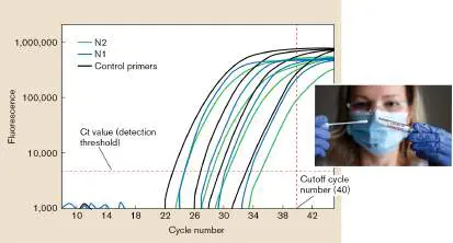
designed to amplify regions of the gene encoding N (nucleocapsid) protein. Each amplification cycle leads to release of a hybridized probe and activation of fluorescence. Inset: Nasal swab sample for COVID-19 PCR test. Ct value = cycle number.
VYACHESLAV LOPATIN/ALAMY STOCK PHOTO
22.3 The Nitrogen Cyclenot assigned
Besides carbon, oxygen, and hydrogen, another major element that cycles largely by microbial conversion is nitrogen (Fig. 22.17). The nitrogen cycle is notable for its dependence on prokaryotes; several steps of the cycle, such as N 2 fixation and nitrous oxide production, are performed solely by bacteria and archaea. Nitrogen cycles are highly perturbed by human technology. About half of atmospheric nitrogen is now fixed into agricultural fertilizer by human chemical factories. The excess reduced nitrogen is then oxidized by lithotrophic microbes (see Chapter 14), some of which release nitrous oxide, a greenhouse gas.
FIGURE 22.17 ■ The global nitrogen cycle. Bacteria and archaea interconvert forms of nitrogen throughout the biosphere.
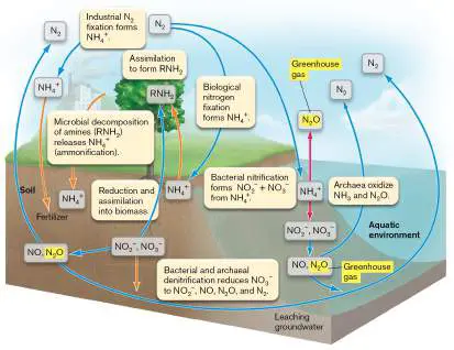
Blue = reduction; red = oxidation; orange = nitrogen available for biomass assimilation.
Sources of Nitrogen
Nitrogen is found in Earth’s crust, in the form of ammonium salts in rock (Fig. 22.2B). Until recently, the nitrogen found in rock was thought to be inaccessible to the biosphere. In 2018, Ben Houlton and Randy Dahlgren at UC Davis showed how up to a quarter of the nitrogen obtained by terrestrial plants could come from weathered rock, in the form of ammonium ion and nitrate. Nonetheless, the largest accessible source of nitrogen is the atmosphere.
The N 2 molecule is highly stable, requiring an enormous input of reducing energy before assimilation is possible (see Chapter 15). Thus, for many natural ecosystems, and most forms of agriculture, nitrogen is the limiting nutrient for primary productivity. Until recently in Earth’s history, N 2 was fixed entirely by nitrogen-fixing bacteria and archaea. In the twentieth century, however, the Haber process was invented for artificial nitrogen fixation to generate fertilizers for agriculture. The process was devised by German chemist Fritz Haber (1868–1934), who won the 1918 Nobel Prize in Chemistry. In the Haber process, N 2 is hydrogenated by hydrogen derived from methane in the form of natural gas. Hydrogenation of N 2 requires extreme heat and pressure. Today, the Haber process for producing fertilizers accounts for approximately 30%–50% of all nitrogen fixed on Earth, and it consumes a substantial portion of fossil fuels. Other human activities, such as fuel burning and use of nitrogenous fertilizers, contribute to oxidized nitrogen pollutants such as nitrous oxide (N 2 O), a potent greenhouse gas (Fig. 22.17, highlighted yellow).
Because of extensive fertilizer use, the nitrogen cycle today is the most perturbed of the major biogeochemical cycles. Half the nitrogen in the biosphere now comes from anthropogenic (human-generated) sources. The ultimate effects of perturbation are not yet clear. Some models show that increased nitrogen fixation could amplify CO 2 fixation by marine and terrestrial ecosystems, partly decreasing net CO 2 emissions. The amount, however, will be too small to prevent global warming. Other models show that accelerated nitrogen use could limit nitrogen availability in the global biosphere, with unknown consequences.
Oxidation States: The “Nitrogen Triangle”
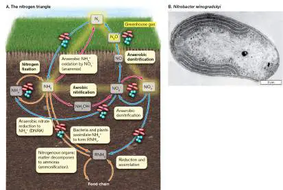
Biological nitrogen exists in a larger number of redox states than does any other element (Table 22.2). The multiple oxidized forms of nitrogen available for microbial metabolism generate a complex cycle of conversions. We can envision a “nitrogen triangle” (Fig. 22.18A) whose corners include three key oxidation states. At the base of the triangle, both reduced and oxidized forms of nitrogen are assimilated into biomass:
Oxidation States of Nitrogen
TABLE 22.2
Compounds
Oxidation state Nitrogen molecule −3 NH, NH + Ammonia,
3 4
ammonium ion −2 H 2 N–NH 2 Hydrazine −1 NH 2 OH Hydroxylamine
Oxidation States of Nitrogen
TABLE 22.2
Compounds
Oxidation state Nitrogen molecule 0 N 2 Nitrogen +1 N 2 O Nitrous oxide +2 NO Nitric oxide +3 HNO, NO − Nitrous acid, nitr
2 2
ite ion +4 NO 2 Nitrogen dioxide +5 HNO, NO − Nitric acid, nitr
3 3
ate ion FIGURE 22.18 ■ The nitrogen cycle: microbial N 2 fixation, nitrification, denitrification. A. The “nitrogen triangle” consists of nitrogen fixation and assimilation, oxidation (nit rification; red arrows), and reductive dissimilation of nitrate (denit rification; blue arrows). Denitrification includes production of the potent greenhouse gas nitrous oxide (N 2 O). Orange arrows = nitrogen available for biomass assimilation.
Assimilation into biomass is often reductive; virtually all nitrogen in biomolecules is highly reduced. Oxidation of ammonia generates nitrites and nitrates, whose runoff can pollute water supplies. DNRA = dissimilatory nitrate reduction to ammonia. B. Nitrobacter winogradskyi oxidizes nitrite to nitrate. Folded layers of membrane contain the electron transport complexes.
SCIENCE VU/S. WATSON/VISUALS UNLIMITED, INC.
NH 3 , fully reduced (ammonia, which ionizes to ammonium ion, NH +)
4
NO − , fully oxidized (nitrate)
3
N 2 , oxidation state of zero (nitrogen gas)
Thought Question
22.3 Which kinds of biomolecules can you recall that contain nitrogen? What are the usual oxidation states for nitrogen in biological molecules?
The three sides of the nitrogen triangle are defined by these microbial reactions: N fixation (reduction) to NH + , a form assimilated into
2 4
biomass by microbes and plants.
Ammonia (NH) oxidation to nitrite (NO −) and
3 2
nitrate (NO −). Nitrite and nitrate can then be assimilated
3
by microbes and plants. Aerobic oxidation to nitrite or nitrate is called nitrification. In anoxic habitats, an aerobic NH 3 oxidation by nitr ite generates N 2 —a reaction called anammox (see Chapter 14).
Denitrification of NO − and NO – back to N (or, in
2 3 2
carbon-rich habitats, microbial reduction by anaerobic respiration to NH 3).
Nitrogen fixation. The main avenue for entry of nitrogen into the biosphere is bacterial and archaeal nitrogen fixation —specifically, fixation of dinitrogen, or nitrogen gas (N 2), into NH 3. (At neutral pH, most of NH is protonated to NH +). Ammonium ion is rapidly
3 4
assimilated by bacteria and plants, typically by combination with tricarboxylic acid (TCA) cycle intermediates such as 2-oxoglutarate, to form key amino acids such as glutamate and glutamine (discussed in Chapter 15). Most kinds of living organisms can assimilate NH + into nitrogenous organic molecules.
4
Fixation of nitrogen requires enormous energy because the triple bond of N 2 is exceptionally stable. Breaking the triple bond to generate ammonia requires a series of reduction steps involving high input of energy: All the intermediate reactions of nitrogen fixation are tightly coupled, so the intermediate compounds rarely become available for other uses. The final product, ammonia, exists in ionic equilibrium with ammonium ion: NH + H O ⇌ NH + + OH −
3 2 4
Half the ammonia is protonated at about pH 9.3, so at near-neutral pH, most of it exists in the protonated form, NH +.
4
Nitrogen fixation is catalyzed by the enzyme nitrogenase (discussed in Chapter 15). The highly reductive reactions of nitrogenase require exclusion of oxygen, yet they also require a tremendous input of energy, usually provided by aerobic metabolism. Therefore, nitrogen-fixing bacteria generally isolate anaerobic nitrogen fixation from aerobic metabolism by one of several mechanisms, such as the heterocysts of cyanobacteria (also discussed in Chapter 15).
Given the energy expense and the need to exclude oxygen, many species of bacteria, as well as all eukaryotes, lack the nitrogen fixation pathway. But all ecosystems, both aquatic and terrestrial, include some species of bacteria and archaea that fix N 2 into ammonia. Nitrogen-fixing bacteria in the soil include obligate anaerobes, such as Clostridium species, and facultative Gram-negative enteric species of Klebsiella and Salmonella, as well as obligate respirers such as Pseudomonas. Marine nitrogen fixers include cyanobacteria such as some species of Trichodesmium. The rhizobia form nitrogen-fixing endosymbionts of legume plants. After fixation, all these organisms assimilate the reduced nitrogen into essential components of their cells. Within an ecosystem, nitrogen fixers ultimately make the reduced nitrogen available for assimilation by nonfixing microbes and plants, either directly through symbiotic association (such as that of rhizobia and legumes, discussed in Chapter 21) or indirectly through predation (marine cyanobacteria) and decomposition (soil bacteria).
If nitrogen fixation is ubiquitous in soil and water, then why is nitrogen limiting? Nitrogen fixation is extremely energy intensive; thus, the rate of fixation usually fails to meet the potential demand of other members of the ecosystem. An exception is legume symbiosis with rhizobia, which provide ample nitrogen for their hosts.
In agriculture, symbiotic nitrogen fixation by rhizobial bacteria increases the yield of crops such as soybeans (Fig. 22.19A). To enhance colonization by nitrogen fixers, farmers apply molecules called isoflavonoids, which mimic the natural plant-derived attractants for rhizobia.
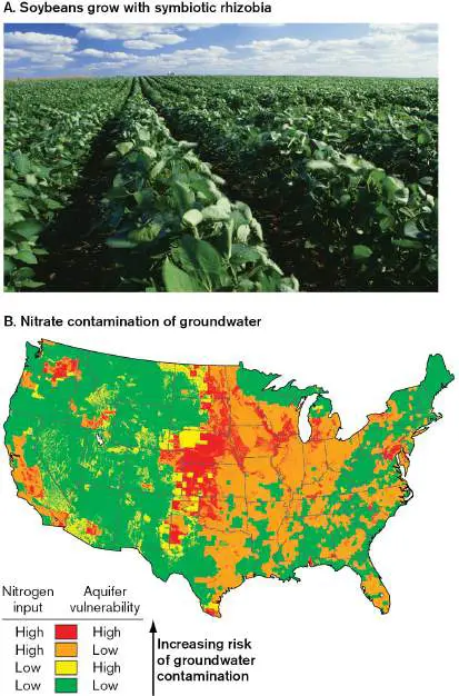
FIGURE 22.19 ■ Agricultural benefits and consequences of microbial nitrogen metabolism. A. Soybean field in Maine. Rhizobial nitrogen fixation enhances growth of soybeans and other major crops. B. Agricultural fertilization releases ammonium, converted by lithotrophs to nitrate, which enters the water supply. Nitrate in drinking water is especially prevalent in agricultural regions of the United States. Nitrate and nitrite runoff from oxidized nitrogenous fertilizers pollutes streams and groundwater.
Source: U.S. Geological Survey, 1999.
GRANT HEILMAN PHOTOGRAPHY/ALAMY STOCK PHOTO
Thought Question
22.4 The nitrogen cycle has to be linked with the carbon cycle, as both contribute to biomass. How might the carbon cycle of an ecosystem be affected by increased input of nitrogen?
Nitrification. Free ammonia in soil or water is quickly oxidized for energy by nitrifiers, bacterial species that possess enzymes for oxidation of ammonia to nitrite (NO −) or of nitrite to nitrate (NO
2 3
−). This process is called nitrification. Nitrification of ammonia is a form of lithotrophy, an energy generation pathway involving oxidation of minerals. The nitrification pathway generates the red base of the triangle in Figure 22.18A. The pathway of nitrification includes: The nitrification pathway contains two separate energy generation mechanisms: (1) ammonia through NH 2 OH to nitrite, and (2) nitrite to nitrate. Typically, soil contains both kinds of microbes, collaborating to complete the conversion to nitrate, while some species of Nitrospira perform the entire pathway, oxidizing ammonia to nitrate. Nitrifying genera include Nitrosomonas, which oxidizes ammonia to nitrite, as well as Nitrobacter (Fig. 22.18B ) and Nitrospira, which oxidize nitrite to nitrate. Nitrite can also serve as an electron donor for photosynthesis by Thiocapsa species. Note that the production of both nitrite and nitrate generates acid, which can acidify the soil.
Thought Question
22.5 In the laboratory, which bacterial genus would likely grow on artificial medium including NH 2 OH as the energy source: Nitrosomonas or Nitrobacter? Why?
Nitrate produced in the soil is assimilated by plants and bacteria nearly as quickly as ammonium ion, although extra energy is needed to reduce nitrate to NH + for incorporation into biomass. Nitrate
4
assimilation to biomass is called assimilatory nitrate reduction. Assimilatory nitrate reduction differs from the nitrate reduction involved in anaerobic respiration, which releases the reduced nitrogen and yields energy. In agriculture, intensive fertilization generates a large excess of ammonia resulting from ammonification, the breakdown of organic nitrogen by catabolism. Catabolism may release ammonia. Ammonia is oxidized rapidly by lithotrophic bacteria (nitrifiers)—a dissimilatory reaction. The excess ammonia leads to a buildup of nitrites and nitrates, which are highly soluble in water, and they readily diffuse into aquatic systems. Aquatic nitrate reacts with organic compounds to form toxic nitrosamines. Nitrate influx also relieves the nitrogen limit on algae, causing algal blooms and raising BOD. Chronic nitrate influx leads to eutrophication and die-off of fish.
Consumption of nitrate in drinking water can lead to methemoglobinemia, a blood disorder in which hemoglobin is inactivated. Methemoglobinemia is a problem for infants because their stomachs are not yet acidic enough to inhibit growth of bacteria that convert nitrate to nitrite. Nitrite oxidizes the iron in hemoglobin, eliminating its capacity to carry oxygen. The failure to carry oxygen leads to a bluish appearance—one cause of “blue baby syndrome.” Nitrite-induced blue baby syndrome is a problem in intensively cultivated agricultural regions, such as Kansas and Nebraska (Fig. 22.19B ).
Agricultural runoff also contributes to oxygen minimum zones and dead zones, such as those off the Oregon coast and in the Gulf of Mexico. The amines in sewage are removed as ammonia (ammonification), and the ammonia is oxidized by lithotrophs. The major marine ammonia oxidizers include the Thaumarchaeota, such as Nitrosopumilus (discussed in Chapter 19).
Denitrification. N 2 is regenerated by anaerobic respiration (Fig. 22.18A), in which an oxidized form of nitrogen, such as nitrate or nitrite, receives electrons from organic electron donors (dissimilatory nitrogen reduction). Bacteria and archaea reduce nitrate through a series of decreased oxidation states back to atmospheric nitrogen: Nitrous oxide Dinitrogen N 2 O + H 2 O ⟶ N 2 + H 2 O + 2H + + 2 e − In terms of elemental flux through ecosystems, nitrate and nitrite reduction are known as denitrification, or dissimilatory nitrate reduction. (In contrast, assimilatory nitrate reduction incorporates nitrogen into biomass.) Many anaerobic respirers in soil or water use an oxidized form of nitrogen as an alternative electron acceptor in the absence of O 2 (discussed in Chapter 14). All types of nitrogen-based anaerobic respiration are repressed in the presence of oxygen, a more favorable electron acceptor; therefore, denitrification is limited to anoxic habitats.
In undisturbed environments, the products of nitrate respiration rarely build up to levels that harm the ecosystem. Heavy fertilization, however, causes buildup of excess nitrate and so increases the environmental rate of denitrification. During this
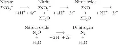
process, some of the nitrogen escapes as nitrous oxide gas (N 2 O). N 2 O is also produced by ammonia-oxidizing bacteria and archaea. A highly potent greenhouse gas, N 2 O generates 200 times the warming effect of CO 2; thus, relatively small amounts of N 2 O can make a disproportionate contribution to global warming.
Furthermore, N 2 O in the upper atmosphere reacts catalytically with ozone, depleting the ozone layer. Thus, the atmospheric effects of microbial denitrification and ammonia oxidation to N 2 O are a serious concern in agricultural and waste treatment processes. Nitrous oxide also builds up in marine dead zones, where the nitrates from ammonium oxidation are subsequently used as electron acceptors. Syed Wajih Naqvi and colleagues at the National Institute of Oceanography in Goa, India, investigated denitrification in the zone of hypoxia off the coast of India (Fig. 22.20A). The study revealed unexpectedly high levels of N 2 O production at a series of stations within the zone. In one experiment, introduction of nitrate into water samples from the dead zone led quickly to production of nitrite and N 2 O (Fig. 22.20B ), a process conducted by denitrifying bacteria. N 2 O is also produced by ammonia-oxidizing archaea such as Nitrosopumilus. Thus, bacterial denitrification and archaeal ammonia oxidation in polluted ocean waters may contribute significantly to global warming.
FIGURE 22.20 ■ Microbial N 2 O production from a coastal dead zone. A. Zone of hypoxia off the coast of India. Circles represent sample-collection stations. B. Levels of NO −,
3
NO −, and N O following addition of NO − to a water sample
2 2 3
from the zone of hypoxia. The sequential rise of NO − and N O
2 2
indicates metabolism by denitrifying bacteria.
Dissimilatory nitrate reduction to ammonia. Most environmental nitrate and nitrite are reduced via N 2 O as described previously. Certain conditions, however, favor the alternate route of dissimilatory nitrate reduction to ammonia (DNRA; see Fig. 22.18A ). Nitrate reduction to ammonia is a form of anaerobic lithotrophy in which nitrate serves as an electron acceptor. An electron donor such as hydrogen gas (H 2) reduces nitrate as follows: NO − + 4H + H + ⟶ NH + 3H O
3 2 3 2
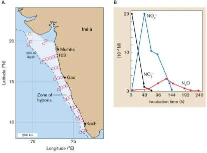
Bacteria reduce nitrate to ammonia mainly in anaerobic environments rich in organic carbon and H 2 generated by fermentation but low in reduced nitrogen—such as sewage sludge and stagnant water. Another carbon-rich habitat favoring this pathway is the rumen, the digestive tract of cattle, goats, and other ruminant animals (see Chapter 21). Ruminants consume grasses whose cellulose requires digestion by mutualistic microbes. Ruminants also depend on their digestive microbes to assimilate nitrate into ammonia and synthesize amino acids.
Anaerobic ammonium oxidation (anammox). For many years, denitrification was considered the main way that nitrogen compounds return N 2 to the atmosphere. In 2003, two research groups from Europe and Costa Rica, led by Tage Dalsgaard and Marcel Kuypers, showed that in anoxic deep-sea water the major source of N 2 is bacteria conducting anaerobic ammonium oxidation by nitrite (the anammox reaction, discussed in Chapter 14): NH + + NO − ⟶ N + 2H O
4 2 2 2
In the anammox reaction, ammonium ion serves as electron donor, and nitrite serves as anaerobic electron acceptor—an unusual combination of two different oxidation states of the same key element, nitrogen. The reaction is a kind of anaerobic lithotrophy. Anammox is performed by bacteria in all kinds of anaerobic habitats, including terrestrial soil and aquatic sediment. The reaction accounts for a majority of all N 2 returned to the atmosphere. Among bacteria, the main anammox contributors are planctomycete genera such as Kuenenia and Scalindua (Fig. 22.21). Anammox planctomycetes (discussed in Chapter 18) are an unusual kind of cell wall–less bacteria with a special interior membrane that segregates the toxic intermediates of the anammox reaction. Promising anammox microbes have been identified from wastewater sludge, in the hope of using them for more effective removal of excess nitrogen from wastewater.
FIGURE 22.21 ■ Anammox bacterium: Scalindua. The planctomycete Scalindua has interior compartments to undergo anammox lithotrophy (discussed in Chapter 14; TEM).
T. AWATA ET AL. 2013. APPL. ENVIRON. MICROBIOL. 79 :4145, FIG. 2A
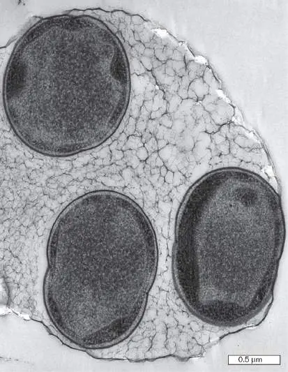
To Summarize
Nitrogen in ecosystems is found in many different oxidation states. Interconversion of most oxidation states requires bacteria or archaea. The nitrogen triangle includes conversions among NH (fully reduced), NO − (fully
3 3
oxidized), and N 2 (oxidation state is zero).
The main source and sink of nitrogen is the atmosphere. N is fixed into NH + by some bacteria and
2 4
archaea. Denitrifying bacteria reduce NO − successively back
3
to N 2 and return it to the atmosphere.
Nitrogen fixation is conducted by symbiotic bacteria in association with specific plants. Legume-associated nitrogen fixation is critical for agriculture.
Nitrification (NH + → NO − → NO − ) is aerobic
4 2 3
oxidation of ammonia to nitrite and nitrate. Nitrification yields energy for lithotrophic bacteria and archaea in soil and water and consumes oxygen, thus expanding marine oxygen minimum zones. Ammonia oxidation also produces nitrous oxide (N 2 O) a potent greenhouse gas.
Bacteria conduct anaerobic respiration , reducing nitrate to N and nitrous oxide. In the deep ocean, NO − may be
2 3
reduced by hydrogen gas to NH 3.
Under anoxic conditions, bacteria oxidize NH + with
4
NO −, generating nitrogen gas (the anammox
2
reaction).
Glossary
nitrogen fixation The ability of some prokaryotes to reduce inorganic diatomic nitrogen gas (N) to two ammonium ions (2NH +).
2 4
nitrifier An organism that converts reduced nitrogen compounds to nitrite or nitrate.
nitrification The oxidation of reduced nitrogen compounds to nitrite or nitrate.
assimilatory nitrate reduction The uptake of nitrate and reduction to NH + by plants, fungi,
4
archaea, and bacteria for use in biosynthetic pathways. ammonification The generation of ammonia from organic nitrogen.
denitrification Also called dissimilatory nitrate reduction. Energy-yielding metabolism in which nitrate (NO −) is reduced to nitrite (NO
3 2
−), diatomic nitrogen (N), and in some cases ammonia (NH
2 3
).
dissimilatory nitrate reduction See denitrification .
anammox reaction The anaerobic oxidation of ammonium to nitrogen gas, using nitrite as electron acceptor; yields energy.
Fig. 22.2B FIGURE 22.2 ■ Global reservoirs of carbon and nitrogen. A. The largest reservoir of carbon is Earth’s crust, but carbon cycles through the biosphere extremely slowly. The major reservoirs for cycling are marine inorganic carbon (CO 2 and carbonates), atmospheric CO 2, and buried fossil fuels. Inset: Marine phytoplankton fix much of Earth’s CO 2. B. The largest reservoirs of nitrogen are atmospheric N 2 and Earth’s crust. Numbers represent the proportion of total global carbon and nitrogen, respectively.
Source: Part B modified from R. Maier et al. 2000. Environmental Microbiology. Academic Press.
ELIF BAYRAKTAR/SHUTTERSTOCK
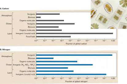
22.4 Sulfur, Phosphorus, and Metalsnot assigned
Besides carbon and nitrogen, many other elements participate in biochemical cycles that have important consequences for the biosphere, as well as for human environments. Sulfur is a major component of biomass, including proteins and cofactors. Like carbon and nitrogen, sulfur can be assimilated in either mineral or organic form. At the same time, assimilation competes with dissimilation by reactions yielding energy, such as sulfide oxidation. Phosphorus, unlike other biological elements, is generally assimilated in the oxidized state, and phosphate is often a limiting nutrient for plants. Iron cycles in complex interactions with sulfur and phosphate. Beyond these macronutrients, many toxic metals in the environment, such as mercury and arsenic, are either bioactivated or detoxified by microbes.
The Sulfur Cycle
Sulfur undergoes a “triangle” of redox conversions analogous to that of nitrogen (Table 22.3). The major redox states are: H S and SH −, fully reduced (sulfides)
2
S 0, oxidation state of zero (elemental sulfur)
SO 2−, fully oxidized (sulfate ion)
4
Oxidation States of Sulfur
TABLE 22.3
Compounds
Oxidation state Sulfur molecules −2 H S, HS − Sulfides
2
0 S 0 Elemental sulfur +2 S O 2− Thiosulfate
2 3
+4 SO 2− Sulfite
3
+6 H 2 SO 4, SO 4 Sulfuric acid, 2− sulfate Reduced forms of sulfur offer electron donors for lithotrophy; these energy-yielding reactions are dissimilatory. H S and SH − can
2
also participate in photolysis through reactions analogous to those of H 2 O (see Chapter 14). Oxidized forms of sulfur such as sulfate, sulfite, and thiosulfate serve as electron acceptors for anaerobic respiration. As we saw for nitrogen, most of these redox reactions are performed solely by bacteria and archaea. The biochemistry of sulfur cycling has important consequences for our “built environment,” such as the corrosion of concrete and iron (discussed shortly).
In the ocean, sulfate is the second most common anion after chloride. Marine sulfate turns over slowly and constitutes an essentially limitless supply. Thus, sulfur is rarely a limiting nutrient. Marine algae release various reduced forms of sulfur, such as dimethylsulfoniopropionate (DMSP). Bacteria metabolize DMSP to dimethyl sulfide [(CH 3) 2 S], which causes part of the “salty sea smell.” Dimethyl sulfide enters the atmosphere, where it becomes oxidized to aerosols that may help water condense and form clouds. In the atmosphere, the overall amount of sulfur (mainly sulfur dioxide) is small. Nevertheless, some sulfur compounds generate toxic effects, as well as acidic pollution. Thus, both biochemical and industrial sources of atmospheric sulfur are of concern.
Assimilatory and dissimilatory sulfur reactions by microbes interconvert H S, S 0, and SO 2− (Fig. 22.22A
2 4
). The “triangle” of oxidation and reduction pathways is analogous to that of nitrogen (compare Fig. 22.18A). Bacterial sulfur metabolism includes additional options of anaerobic phototrophy, such as H 2 S phototrophy. In an aquatic system, H 2 S arises from spring waters welling up from the sediment and from decomposition of detritus. During decomposition, anaerobic respirers such as Desulfovibrio s pecies convert sulfate to sulfur, then to H 2 S. As H 2 S rises to the oxygenated surface water, it is readily oxidized by sulfur-oxidizing bacteria such as Acidithiobacillus and Beggiatoa.
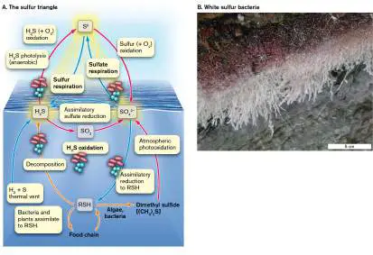
FIGURE 22.22 ■ The sulfur cycle. A. The “sulfur triangle.” In the presence of oxygen, bacteria and archaea oxidize H 2 S to sulfur dioxide, and then to sulfate. Anaerobically, H 2 S may be photolyzed to sulfur. Sulfate serves as an electron acceptor for anaerobic respiration or it may be assimilated into biomass as reduced sulfur groups (RSH). Algae form DMSP (dimethylsulfoniopropionate), which bacteria convert to dimethyl sulfide. Arrows: blue = sulfur reduction; red = sulfur oxidation; orange = redox-neutral sulfur conversion. B. Microbial mat of white, sulfur-oxidizing bacteria (probably Beggiatoa) growing at a sulfide spring.
DR. JUERGEN SCHIEBER, INDIANA UNIVERSITY DEPARTMENT OF GEOLOGICAL
SCIENCE
Beggiatoa species are known as “white sulfur bacteria” because they form white mats (Fig. 22.22B ). Their appearance is due to the sulfur granules generated by sulfide oxidation. Microbial sulfide oxidation is helpful for environments because it removes H 2 S, which is highly toxic to most nonsulfur bacteria and plants. Because of the toxicity of H S, autotrophs more readily assimilate SO 2−
2 4
into biomass, despite the extra energy needed to reduce SO 2− to
4
the thiol form found in proteins.
If light is available, anaerobic phototrophs such as Rhodopseudomonas species will use light energy to oxidize H 2 S. Some phototrophic bacteria further oxidize the S 0 generated to sulfate. In some sulfur-rich lakes, such as Russia’s Lake Sernoye, underground springs pump in so much H 2 S that most of the sulfur is photolytically converted to S 0, which forms up to 5% of the sediment. This elemental sulfur can be mined commercially. In thermal vent ecosystems, several sulfur-based reactions drive metabolism. For example, thermal vent archaea such as Pyrodictium species use sulfur to oxidize hydrogen gas to H 2 S: H + S 0 ⟶ H S
2 2
This type of sulfur-based hydrogenotrophy is enhanced by the vent conditions of extreme pressure and temperature (100°C). Acid conditions (pH < 4) also enhance sulfur reduction by hyperacidophilic archaea.
Decomposition of biomass generates various organic sulfur compounds, many of which are volatile. Odors of certain microbial sulfur products contribute to the smell of rotting eggs, but others enhance the taste of cheeses (discussed in Chapter 16).
Sulfur is reduced by sulfur-reducing bacteria in many subsurface environments, such as beneath deposits of oil and coal (Fig. 22.23A). Oil and coal contain sulfur in the form of SO 2− and
4
provide a carbon source for sulfate respirers (sulfate-reducing bacteria that respire using sulfate as a terminal electron acceptor). The products of sulfate respiration include S 0 and organic sulfur. When the fuel is burned, these forms of sulfur cause severe pollution. Before burning, however, the S 0 and organic sulfur can be oxidized by sulfur-oxidizing bacteria. Fuel processors are now turning to sulfur-oxidizing microbes for experimental use in “desulfuration,” the removal of sulfur from coal.
FIGURE 22.23 ■ Consequences of the microbial sulfur cycle. A. Oil-or coal-bearing geological strata provide rich
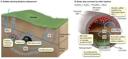
electron donors for sulfate-reducing bacteria (sulfate respirers). Eventually, various forms of sulfur contaminate the oil or coal, which, when burned as fuel, generates first SO 2 and ultimately sulfuric acid (acid rain). B. In a sewer pipe, sulfate-reducing bacteria (sulfate respirers) generate H 2 S. Sulfur-oxidizing bacteria then oxidize H 2 S to sulfate in the form of sulfuric acid. The sulfuric acid reacts with calcium hydroxide in the concrete, thus corroding the interior surface of the pipe.
One habitat that exhibits the entire range of sulfur oxidation states is a sewer pipe. In a concrete sewer pipe, the alternation between anaerobic and oxygenated sulfur biochemistry causes severe corrosion (Fig. 22.23B ). The microbial decomposition of sewage yields large quantities of toxic H 2 S, which then volatilizes to high levels that endanger sewer workers. The H 2 S is then oxidized to sulfuric acid by Acidithiobacillus ferrooxidans, a bacterium that colonizes the surface of the concrete. The sulfuric acid (H 2 SO 4) decreases the pH at the concrete surface to pH 2. In the concrete surface, sulfuric acid converts calcium hydroxide to calcium sulfate, which dissolves in water. Over several years, this corrosion can eat away half the thickness of a sewer pipe. Sulfur metabolism shows important connections with metabolism of metals. For example, sulfur-oxidizing bacteria such as A. ferrooxidans oxidize iron as well (discussed shortly).
Thought Question
22.6 Compare and contrast the cycling of nitrogen and sulfur. How are the cycles similar? How are they different?
The Phosphate Cycle
Phosphorus is a fundamental element of nucleic acids, phospholipids, and phosphorylated proteins. Unlike sulfur and nitrogen, which are found in several different oxidation states, phosphorus is cycled mainly in the fully oxidized state of phosphate ( Fig. 22.24). The absence of fully reduced phosphorus in ecosystems may be due to the fact that reduced phosphorus (phosphine, PH 3) undergoes spontaneous combustion in the presence of oxygen. Nevertheless, some anaerobic decomposers use phosphate as a terminal electron acceptor, reducing it to phosphine. In marshes and graveyards, where extensive decomposition occurs, phosphine emanates from the ground, where it ignites with a green glow. Microbial respiration of phosphate might be the cause of such “ghostly” apparitions.
FIGURE 22.24 ■ The phosphate cycle. Phosphorus in the biosphere occurs entirely in the form of inorganic or organic phosphate. Most phosphate precipitates as insoluble salts in
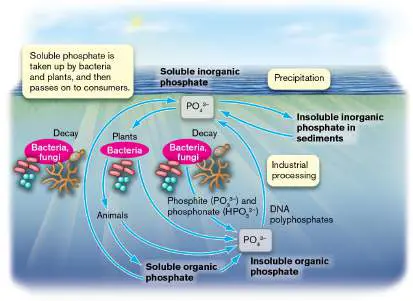
sediment. The small amount of soluble phosphate is taken up by plants and bacteria, which may then be taken up by consumers. Decomposers return phosphate to the environment.
Where is phosphate available? Although phosphate is abundant in Earth’s crust, its availability in ecosystems is limited by its tendency to precipitate with calcium, magnesium, and iron ions. Thus, dissolved phosphate in water and soil is often a limiting nutrient for productivity. In natural ecosystems, the available phosphate is taken up rapidly by bacteria and phytoplankton, and then consumed by grazers and predators and dispersed by decomposers.
Marine water is extremely limited for phosphate, because of the distance from sediment minerals. Thus, the genomes of marine phototrophs encode many systems for acquiring phosphate from organic sources. Some actually acquire phosphorus in a partly reduced form, such as phosphite (PO 3−) or phosphonate (HPO
3 3
2−), both of which are available in marine water. In addition, marine phototrophs show an unusual ability to substitute nonphosphorus lipids for phospholipids, thus cutting their phosphorus needs by half. For example, the cyanobacteria Prochlorococcus, Synechococcus, and Trichodesmium can replace membrane phospholipids with sulfonated lipids. Similarly, algae such as Thalassiosira species can replace phosphatidylcholine with betaine, which contains no phosphate but includes a carboxylate group.
Another microbial response to phosphate scarcity is to replace membrane phosphates with organic phosphonates, in which the phosphorus atom bonds directly to carbon (R–PO 2−), instead of
3
via the easily hydrolyzed phosphoester bond. These organic phosphonates, however, are cleaved by marine archaea, the ammonia oxidizers such as Nitrosopumilus. The archaea release methylphosphonate, which many bacteria can cleave to obtain phosphate. Phosphate scavenging from methylphosphonate releases methane, thus interacting with the carbon cycle.
In agriculture, phosphate is often added as a fertilizer. Phosphate fertilizer is obtained by treating calcium phosphate rock with sulfuric acid, producing calcium sulfate (gypsum) and phosphoric acid. Excess phosphate from fertilizer or industry may drain into streams and lakes where phosphorus is the limiting element. The sudden influx of phosphate causes an algal bloom. The overgrowth of algae leads to overgrowth of heterotrophs, depletion of oxygen, and destruction of the food chain.
Thought Question
22.7 Compare and contrast the cycling of nitrogen and phosphorus. How are the cycles similar? How are they different?
The Iron Cycle
Why do organisms need iron? As a micronutrient, iron forms a negligible part of biomass but is essential for growth (discussed in Chapter 4). Organisms require iron as a cofactor for enzymes and an essential component of oxygen carrier molecules such as hemoglobin. Other common micronutrients required for enzymes and cofactors are zinc, copper, and selenium.
Iron is a major component of Earth’s crust, and substantial quantities are present in most soil and aquatic sediment. Yet the availability of iron to organisms is limited by its extremely low solubility in the oxidized form. In microbial biochemistry, the oxidized form, ferric iron (Fe 3+), interconverts with the reduced form, ferrous iron (Fe 2+; Fig. 22.25A). In the presence of oxygen, iron metal (Fe 0) “rusts” and is therefore available to organisms mainly as Fe 3+. Ferric iron is especially insoluble at high pH, precipitating with hydroxide ions as ferric hydroxide [Fe(OH) 3] or with phosphate ions as ferric phosphate (FePO 4). At neutral pH, iron is oxidized by bacteria such as Gallionella, Leptothrix, and Mariprofundus.
FIGURE 22.25 ■ The iron cycle. A. Ferric iron (oxidized iron, Fe 3+) precipitates with hydroxide or phosphate. Only bacteria can assimilate Fe 3+. In anoxic sediment, bacterial respiration reduces Fe 3+ to Fe 2+, a more soluble form available to plants. Arrows: blue = iron reduction; red = iron oxidation; orange = redox-neutral iron conversion. B. Home plumbing shows signs of lithotrophic oxidation of Fe 2+ to Fe 3+ (orange precipitate).
BRYAN ALLEN
Marine iron. In the upper layers of most oceans, iron is extremely scarce. This is because the benthic sediment containing iron is so distant that its iron is largely inaccessible. The main source of marine iron is eolian (wind-borne) dust from dry land, such as from windstorms in the Sahara desert. Most of the wind-borne iron is particulate, oxidized, and unavailable to eukaryotic phytoplankton
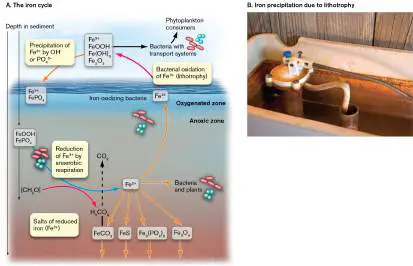
(algae). Thus, bacteria that acquire and reduce ferric iron provide the main entry of iron into the ecosystem. This may explain why so many marine algae are mixotrophs: Although their photosynthesis can fix plenty of carbon for biomass, they consume bacteria as a source of iron. Another source of marine iron is hydrothermal vents. Iron is thus a limiting nutrient for marine phytoplankton. As discussed in Chapter 21, when higher quantities of a limiting nutrient enter an ecosystem, the limited populations rapidly increase. The rise of algal populations following iron addition was demonstrated in an “iron fertilization” experiment conducted in 2007 by Phillip Boyd and colleagues at the University of Otago, New Zealand. Several thousand kilograms of ferrous sulfate (FeSO 4) was released in the Southern Ocean, near Antarctica. Within a week after the iron release, there was a bloom of phytoplankton. The dominant phytoplankton in the bloom were diatoms of the species Fragilariopsis kerguelensis. The diatom bloom was so large that it was detected by a NASA satellite as a region of increased color reflected by chlorophyll.
The dramatic effects of iron fertilization led some researchers to propose that increasing iron throughout the oceans could cause blooms of diatoms, removing CO 2 from the atmosphere. If a sufficiently large proportion of the diatoms were to escape predation and fall to the ocean floor, they would effectively remove their carbon from circulation. An alternative outcome, however, would likely be eutrophication, causing an ecological collapse comparable to a dead zone.
Iron in soil and sediment. In anoxic habitats, such as benthic sediment, Fe 3+ is largely reduced to Fe 2+ by anaerobic respiration. Reduction leads to loss of the reddish color, generating gray-colored sediment, as in wetland soil (discussed in Chapter 21). The reduction of Fe 3+ to Fe 2+ is one of the enriching contributions of anaerobic sediment to freshwater wetlands and coastal estuaries, because reduced iron is more available to plants and bacteria. Oxidized iron, in aerobic soils, can be taken up only by bacteria. Bacteria synthesize special iron uptake systems, including molecules called siderophores that bind ferric ion outside and then are taken up by the cell (see Section 4.2). Bacterial iron then becomes available to consumers in the ecosystem.
In iron mines, where pyrite (FeS 2) is exposed to air, spontaneous oxidation releases sulfuric acid: 2FeS + 7O + 2H O + 4H + ⟶ 2Fe 2+ + 4H SO
2 2 2 2 4
Lithotrophs such as Acidithiobacillus ferrooxidans can use O 2 as terminal electron acceptor for iron oxidation to yield energy, thus increasing the rate of production of sulfuric acid. Rapid sulfuric acid production leads to acid mine drainage. Where acid mine drainage enters an aquatic system, the reduced iron is oxidized by lithotrophs to ferric hydroxide, forming an orange precipitate. A similar precipitate from bacteria in iron-rich water occurs in home plumbing (Fig. 22.25B ). Iron mine drainage causes severe pollution of streams (Fig. 22.26).
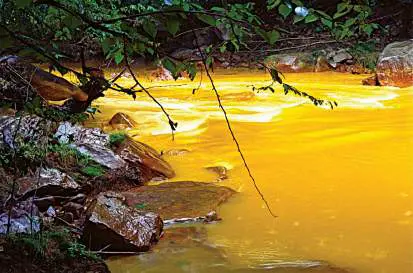
FIGURE 22.26 ■ Mine drainage enters a stream. Lithotrophic oxidation of reduced iron yields the orange material polluting this stream in Preston County, West Virginia.
THOMAS R. FLETCHER/ALAMY
Iron cycling often connects with the sulfur cycle in ways that can prove unfortunate for our built environment. The most serious problem is anaerobic corrosion of iron, such as the iron structures of bridges. Iron corrodes spontaneously in the presence of oxygen. In anoxic environments, however, little spontaneous corrosion takes place. Instead, iron is corroded by sulfate-reducing bacteria (Fig. 22.27). Bacteria such as Desulfovibrio and Desulfobacter can grow on the iron surface, forming an anaerobic biofilm. Within the biofilm, iron is oxidized to Fe 2+, and sulfate dissolved in the water is reduced to ferrous sulfide: FIGURE 22.27 ■ Anaerobic corrosion. Iron-sulfur bacteria convert Fe 0 to FeS. FeS flakes off, exposing iron to further oxidation and rapid corrosion.
Source: Modified from Hang T. Dinh et al. 2004. Nature 427 :829–832.
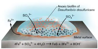
4Fe 0 + SO 2− + 4H O ⟶ FeS + 3Fe 2+ + 8OH −
4 2
The FeS flakes away, exposing more iron to react with water, resulting in cyclic corrosion.
Other Metals in the Environment
Another concern for environmental management is the problem of toxic metals and metalloids such as mercury and arsenic. Besides iron, numerous trace metals interact with bacterial species as either electron donors or acceptors (Table 22.4). Bacterial conversion of metals can either produce toxic species or remove toxic metals from ecosystems. For example, chromium-6 [Cr(VI)] is an extremely toxic pollutant that can be reduced by soil bacteria to the much less toxic Cr(III).
TABLE Microbial Metabolism of Metals 22.4
Microbial Effects Major genera within Metal conversions (examples) environment Arsenic (As) AsO 3− ⟶ Alcaligenes, Oxidation of
3
AsO 3− Pseudomonas poisonous
4 3−
AsO 3 via use as terminal e − acceptor, converting to insoluble AsO 3−.
4
AsO 3− ⟶ Bacillus, Reduction of
4
− Chrysiogenes, AsO 3− AsO 2 4 Pyrobaculum (arsenate)
used as terminal e − acceptor.
AsO 3− ⟶ Candida (a Formation of
4
(CH) fungus), methylarsine
3 3
As Scopulariopsis s. Poisonous; (a fungus) inhalation of moldy wallpaper with arsenic pigment.
Chromium CrO 2− ⟶ Aeromonas, CrO 2−
4 4
(Cr) Cr 3+ Arthrobacter, [Cr(VI)] is Desulfovibrio mutagenic and carcinogenic; as e − acceptor, reduced to Cr 3+ [Cr(III)], less toxic.
Manganese Mn 2+ ⟶ Mn Hyphomicrobium, Mn is a trace (Mn) 4+ Arthrobacter element required for enzymes.
Mn 4+ ⟶ Mn Geobacter, Anaerobic 2+ Pseudomonas respiration in sediment.
Mercury Hg 2+ ⟶ Hg Acidithiobacillus Hg 0 (Hg) 0 volatilizes; little harm.
Hg 2+ ⟶ (CH Desulfovibrio (CH)Hg + is
3
)Hg + a severe
3
neurotoxin; accumulates at higher trophic levels, such as fish.
Selenium Se 0 ⟶ SeO Bacillus, Se is a trace (Se) 2− Micrococcus element;
3
small amounts in food help remove mercury.
Larger amounts are toxic.
Uranium UO 2+ ⟶ Veillonella, UO 2+
2 2
(U) UO Shewanella, [U(VI)],
2
Geobacter soluble, is respired to uranium dioxide, UO 2 [U(IV)], insoluble; used for cleanup of radioactive uranium.
Vanadium VO − ⟶ Veillonella, V is a trace
3
(V) VO(OH) Desulfovibrio, element for Clostridium some nitrogenases and invertebrate blood pigments.
VO −
3
(vanadate)
is oxidized as an e − donor.
How can bioremediation remove toxic minerals from groundwater? Microbial metabolism can convert a toxic metal to an insoluble form, which then precipitates out of groundwater. For example, the anaerobic respiration by Geobacter metallireducens is used to convert toxic uranium ion, U 6+ (VI) to the insoluble form U 4+ (IV). Bioremediation by Geobacter was described in Chapter 14.
Multiple Limiting Factors Modulate Complex Ecosystems
A common assumption of terrestrial and aquatic ecology is that a single nutrient, such as phosphorus or iron, is limiting for a given ecosystem. In marine water, however, more than one factor may be limiting. The requirement for more than one limiting factor is known as resource colimitation. In highly oligotrophic marine water, populations often depend on multiple limiting factors. For example, in the Baltic Sea, both nitrogen and phosphorus are present in such low concentrations that they must be added together in order to stimulate a phytoplankton bloom. In another example, the North Atlantic is limited for both phosphorus and iron. Addition of both P and Fe stimulates growth of nitrogen-fixing cyanobacteria.
To Summarize
Oxidized and reduced forms of sulfur are cycled in ecosystems. Sulfate and sulfite serve as electron acceptors for respiration. Hydrogen sulfide serves as an electron donor. Sulfur oxidation to sulfuric acid causes acid mine drainage and pipe erosion.
Phosphorus cycles primarily in the fully oxidized form (phosphate). Phosphate limits growth of phototrophic bacteria and algae in some freshwater and marine systems. Iron cycles in oxidized and reduced forms. Oxidized iron (Fe 3+) serves as a terminal electron acceptor in anaerobic soil and water. Reduced iron (Fe 2+) from rock is oxidized through weathering or mining. Bacterial lithotrophy accelerates iron oxidation, leading to acidification.
Metal toxicants can be metabolized by bacteria.
Bacterial metabolism may either increase or decrease toxicity. Metabolic conversion to an insoluble form offers an effective means of bioremediation.
Marine habitats show resource colimitation. Multiple resources may be limiting for the phytoplankton community or for different microbial populations.
Glossary
siderophore A high-affinity iron-binding protein used to scavenge iron from the environment and deliver it to a siderophore-producing organism.
resource colimitation A situation in which a population size is limited by the lack of two different resources, such as nitrogen and phosphorus. Fig. 22.18A
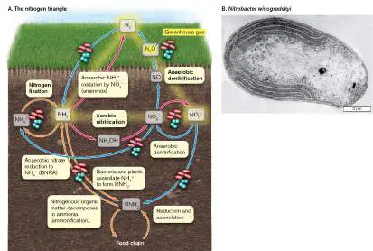
FIGURE 22.18 ■ The nitrogen cycle: microbial N 2 fixation, nitrification, denitrification. A. The “nitrogen triangle” consists of nitrogen fixation and assimilation, oxidation (nit rification; red arrows), and reductive dissimilation of nitrate (denit rification; blue arrows). Denitrification includes production of the potent greenhouse gas nitrous oxide (N 2 O). Orange arrows = nitrogen available for biomass assimilation. Assimilation into biomass is often reductive; virtually all nitrogen in biomolecules is highly reduced. Oxidation of ammonia generates nitrites and nitrates, whose runoff can pollute water supplies. DNRA = dissimilatory nitrate reduction to ammonia. B. Nitrobacter winogradskyi oxidizes nitrite to nitrate. Folded layers of membrane contain the electron transport complexes.
SCIENCE VU/S. WATSON/VISUALS UNLIMITED, INC.
22.5 Our Built Environmentnot assigned
Humans increasingly live in a habitat that was built by our technology, rather than existing in a “natural” environment. In developed countries, people are estimated to spend 90% of their time indoors. By shaping environments for our own comfort and convenience, we unwittingly have shaped the microbial communities that cohabit with us. Microbiologists study our built environment with the aim of understanding how the associated microbial communities interact with human inhabitants, in positive as well as negative ways.
While many microbes contribute to our health, our built environment also concentrates our exposure to human pathogens. The COVID-19 pandemic was amplified by spread of the coronavirus within building interiors. Resulting research points to new ways of decreasing disease by ventilation and air filtration.
The Microbiome of Building Interiors
Built structures include homes, offices, and transportation vehicles such as automobiles and subway cars. Questions we ask about the interiors of such structures include: What kinds of microbes are present? What are the natural or human sources of the microbes? How do the microbes’ activity affect human life?
Figure 22.28presents the results of a study by Marzia Miletto and Steven Lindow at UC Berkeley, in which air was sampled from 29 different home interiors. From the air samples, genes expressing 16S rRNA were amplified and sequenced. In this one study, the most abundant organism found was Diaphorobacter species (Fig. 22.28, inset), family Comamonadaceae. These are betaproteobacteria commonly found in air, water, and soil; they are capable of aerobic or anaerobic catabolism on various substrates. Yet Diaphorobacter represents only 10% of the community found. Other prominent members include Sphingomonadaceae (Alphaproteobacteria) and Propionibacteriaceae, which are actinobacteria that colonize human skin. (see Chapter 18 for a review of bacterial diversity.) FIGURE 22.28 ■ Indoor air microbiome. Air samples from indoor environments in San Francisco were tested for bacterial taxa at the family level. The relative abundance of the top 20 taxa found was compared with respect to the same taxa from other sources. Inset: Diaphorobacter species from a soybean root nodule.
Source: Modified from M. Miletto and S. Lindow. 2015. Microbiome 3 :61, fig. 1.
XIU LI WEI ET AL. 2015. ARCH. MICROBIOL. 197 :683, FIG. 1B
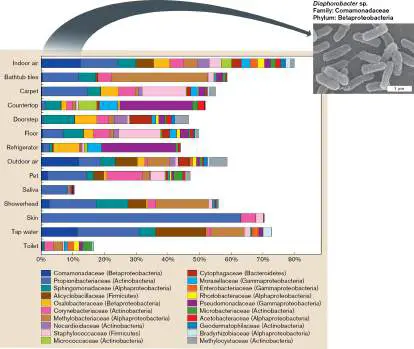
The abundance values of various taxa of indoor air samples were plotted and compared to those from samples of other interior sources, such as human skin, countertops, and tap water. The highest proportions of corresponding taxa were found in outdoor air and tap water. Pet animals showed many taxa in common with those of indoor and outdoor air, including the top five taxa found in indoor air. Pets showed additional taxa not found in air (not shown in Fig. 22.28). Human skin showed one highly represented taxon, the Propionibacteriaceae, which may cause skin infections such as acne. Another airborne taxon shared by human skin was Corynebacteriaceae, a family including commensals, as well as pathogens such as Corynebacterium diphtheriae. Other airborne bacteria do not normally reside in skin. Surprisingly low airborne representation was seen for taxa found in human saliva. Well-ventilated buildings show relatively little airborne content from the human occupants, and they share greater content with external air. Indoor environments vary in their microbial community structure. Environments largely limited to human occupation, such as hospitals and public transport, often show high abundance of bacteria derived from human skin and mucosal sources (Fig. 22.29). These include the genera Staphylococcus and Streptococcus, as well as Cutibacterium. In the home, various common objects may be surprising sources of microbes. A remarkably fertile source is the kitchen sponge (Special Topic 22). Hospitals show additional taxa associated with pathogens, such as Pseudomonas and Acinetobacter.
FIGURE 22.29 ■ Bacteria found in the built environment. Human-built habitats such as hospitals and public transport show distinctive microbial communities that differ from those of farm environments. MRSA = methicillin-resistant Staphylococcus aureus.
Source: Modified from J. A. Gilbert and B. Stephens. 2018. Nat. Rev. Microbiol. 16 :661–670, fig. 1.
An interesting finding is that farms and home spaces exposed to pet animals show a more diverse microbiome with a broader range of harmless, animal-associated taxa such as lactobacilli. Studies suggest that the farm microbiome offers a protective effect against
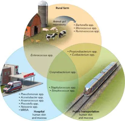
allergies, particularly in children. These findings have led to the “old friends” hypothesis, which proposes that humans evolved in the presence of certain harmless taxa of microbes that increase our health by assisting maturation of the immune system (discussed in Chapter 23). Without these “old friends,” the immune system may be more likely to undergo dysregulation leading to inflammatory diseases. This hypothesis suggests that controlled exposure to farms and pet animals may increase the diversity of health-enhancing microbes in the indoor microbial community.
At the same time, farm microbiomes include exposure to potential pathogens such as Bartonella (cause of cat scratch disease) and Enterococcus. Thus, we need to study the mechanisms of microbial transfer from sources and sinks of harmful microbes and from those of beneficial bacteria.
Airborne Pathogens in Our Built Environment
Historically, our society has expressed great concern over pathogen transmission in water and food. Pathogen removal from waterways is addressed by wastewater treatment (see Section 22.2), and disinfection of food is addressed by food preservatives and sterilization (see Section 16.4). In the United States and other countries, such processes are subject to intense government regulation. Yet, surprisingly, little regulation addresses infection by air. This is the case despite a long history of awareness of airborne infections such as tuberculosis. In the early twentieth century, many European and American communities sought to avoid tuberculosis by conducting public school outdoors. However, the interest in preventing airborne infection was later eclipsed by the greater awareness of poliovirus in water and other pathogens in food.
SPECIAL TOPIC 22 A Microbial Jungle in a Kitchen Sponge
Which object would you guess hosts the largest, most diverse source of bacteria in your home? Many of us would first guess the bathroom toilet. The answer, however, turns out to be the kitchen sponge—the implement we rely on to scrub our pots clean (Fig. ST 22.1 ).
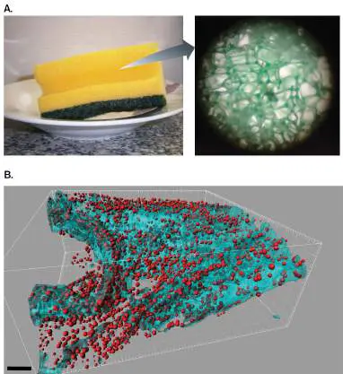
FIGURE ST 22.1 ■ Microbiome of a kitchen sponge. A. Kitchen sponge. Inset: Microscopic view of pores in a sponge sample (LM). B. Kitchen sponge sample, 3D confocal microscopy, with FISH probe detection of Gammaproteobacteria (red) and sponge material autofluorescence (cyan).
M. CARDINALE ET AL. 2017. SCI. REP. 7 :5791, FIG. 1B
M. CARDINALE ET AL. 2017. SCI. REP. 7 :5791, FIG. 1B
M. CARDINALE ET AL. 2017. SCI. REP. 7 :5791, FIG. 4D
Markus Egert (Fig. ST 22.2A ) and colleagues at Hochschule Furtwangen University, Germany, conducted a taxonomic analysis and 3D microscopic visualization of a collection of used kitchen sponges. They reasoned that sponges would act as “microbial incubators,” continually exposed to fresh nutrients, moisture, and microbes from body contact. Figure ST 22.1 (inset) shows the porous form of a sponge, which traps moisture and microbes, no matter how hard the sponge is squeezed out. Egert visualized the sponge samples in 3D, using confocal laser scanning microscopy (described in Chapter 2) combined with fluorescence in situ hybridization (FISH; Chapter 21). The FISH probe (red fluorescence) contained a 16S rRNA gene sequence specific to the Gammaproteobacteria Fig. ST 22.1B ). Thus, we can see that Gammaproteobacteria are widespread throughout the used sponge. Overall, the sponge showed as many as 50 billion bacteria per square centimeter—a density nearly as high as that of human feces.
FIGURE ST 22.2 ■ Markus Egert studies the kitchen sponge microbiome. A. Markus Egert. B. Bacterial taxa detected by sequencing 16S rRNA gene amplicons.
Source: Part B modified from M. Cardinale et al. 2017. Sci. Rep. 7 :5791, fig. 1C.
COURTESY OF MARKUS EGERT
The full taxonomic profile of kitchen sponges, using 16S rRNA gene probes, shows an enormous variety of bacteria from diverse clades (Fig. ST 22.2B ). Dominating the profile were the Gammaproteobacteria, including Escherichia coli and other enteric bacteria. The major family, however, was not Enterobacteriaceae but Moraxellaceae, representing a third of the sponge community. Moraxellaceae includes a respiratory pathogen, Moraxella catarrhalis, but also contains numerous commensals of humans and other animals. Another family abundant in the sponge was Pseudomonadaceae, which may include pathogens and soil-dwelling bacteria.
Egert’s team tested the effectiveness of “special cleaning” procedures such as microwave heating. While microwave cleaning decreased the bacterial content somewhat and
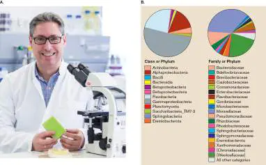
altered the taxa distribution, the sponge samples remained full of bacteria. Cleaned or not, the kitchen sponge retains its title as the most dense and diverse source of bacteria in the human-built environment.
RESEARCH QUESTION
How does the kitchen sponge microbiome interact with that of the home’s human inhabitants? Do sponge microbiomes influence the human microbiome or vice versa?
Cardinale, Massimiliano, Dominik Kaiser, Tillmann Lueders, Sylvia Schnell, and Markus Egert. 2017. Microbiome analysis and confocal microscopy of used kitchen sponges reveal massive colonization by Acinetobacter, Moraxella and Chryseobacterium species. Scientific Reports 7:5791.
Today, the techniques of PCR and nucleic acid sequencing show that our home and office interiors continually acquire microbes from their human inhabitants. A human body may disperse millions of bacteria and fungal spores per hour, many of them airborne, largely via skin contact and shedding of particles. This human spread of microbes is a problem for hospitals, where a patient’s room rapidly acquires the microbiome of its occupant. Hospital microbes commonly include difficult-to-treat pathogens such as methicillin-resistant Staphylococcus aureus (MRSA) and Candida auris, an emerging fungus (Fig. 22.30). Pathogens may be transmitted via inhalation of droplets and desiccated particles from other patients, from hospital staff, or even from the doctor’s necktie.
FIGURE 22.30 ■ Transmission of microbes within the built environment. Microbes may be transmitted from human occupants to the built environment and vice versa. “Fomites” are inert objects that may carry microbes.
Source: Modified from J. A. Gilbert and B. Stephens. 2018. Nat. Rev. Microbiol. 16 :661–670, fig. 2.
The COVID-19 pandemic provided abundant evidence of how a pathogen can be transmitted by air (discussed in Chapter 6). At first, it was thought that the coronavirus particles were carried only by large droplets of respiratory fluid expelled by coughing or sneezing. Close contact is certainly the most efficient route for transmission, but epidemiology showed that, for example, passengers on a cruise ship confined to their cabins nearly all tested positive for coronavirus despite lack of contact with a carrier. This result could best be explained by transmission via the ship’s air
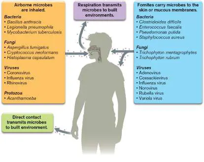
exchange system. The consensus in 2022 is that airborne coronavirus particles may be carried for hours or days on aerosol; that is, air-suspended droplets 5 μm in size or smaller. Note that aerosol transmission depends on the virus. Only certain kinds of viruses, such as coronavirus, influenza virus, and measles virus, survive on airborne droplets.
The pandemic experience has led to a renewed focus on air health and safety in our built environment. Besides microbial pathogens, many particles of allergens and pollutants accumulate in indoor air, leading to a large cumulative burden of disease. How can we make the air we breathe as safe as the water we drink? How can “waste air” be treated?
To decrease aerosol transmission in the built environment, epidemiology supports the value of ventilation, the exchange of indoor air with fresh outdoor air. The increased ventilation of public spaces, including the practice of outdoor dining and schooling, is associated with decreased rate of COVID-19 transmission as well as decreased allergic illness and pollution exposure. Yet ventilation is not always a practical solution, particularly under conditions of extreme cold or heat, and in city environments with high levels of outdoor pollution. Because more polluted urban neighborhoods tend to have higher proportions of members of minority ethnic or racial groups as residents, unhealthy air exposure is one factor contributing to health disparities (see Section 28.6).
Another form of air treatment is air recirculation through a high-efficiency particulate air filter (HEPA filter) of grade 13 (HEPA 13). HEPA 13 filters are certified by government standards to remove at least 99.97% of all airborne particles and droplets of diameter 0.3 μm or larger. They are designated medical-grade. HEPA filters have long been used by industry and medical research to remove harmful particles and pathogens; for example, a laboratory hood used at biosafety level 2 or higher must pass air through a HEPA filter. A portable HEPA filter can be used to recirculate air within a room, thus continually removing harmful particles. During the COVID-19 pandemic, inexpensive HEPA air recirculators became available for consumer use (Fig. 22.31A).
FIGURE 22.31 ■ HEPA filter air recirculation decreases aerosol transmission of pathogens. A. An inexpensive home air recirculator with a HEPA filter. HEPA filtration removes aerosol droplets containing pathogenic microbes. B. An experiment tests the effectiveness of HEPA filtration in a hospital ward housing SARS-CoV-2 patients. Air was sampled from a four-bed ward with a HEPA air recirculator turned off or turned on. Air was collected on sample filters with a flow rate of 3.5 l/min for 6 hours; microbes were detected by taxa-specific PCR. When the recirculator was turned on, only a small fraction of airborne pathogens were detected, compared to those found when the recirculator was off.
Source: Modified from Andrew Conway Morris et al. 2022. Clinical Infectious Diseases 75 :e97-e101.
GADO IMAGES/ALAMY STOCK PHOTO
Do HEPA filters actually remove pathogens? An experiment by Andrew Conway Morris and colleagues from Cambridge University hospitals in the United Kingdom put HEPA 13 air recirculators to the test (Fig. 22.31B ). For this experiment, a HEPA air recirculator was placed in a four-bed hospital ward (air volume, 107 cubic meters) where all patients tested positive for SARS-CoV-2. The air flow rate was set at 1,000 cubic meters per hour, which was
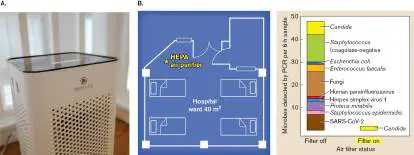
sufficient to filter all the air in the room several times per hour. The air was sampled and filtered by a U.S. National Institute for Occupational Safety and Health (NIOSH) aerosol collector at 3.5 l/min for 6 hours. Sampling was performed with the HEPA unit turned on or off, and replicate trials were conducted. The collection filters were assayed by PCR for ten microbial taxa, including representative bacterial, viral, and fungal pathogens. Results showed that the filter unit removed more than 99% of most kinds of pathogens, including SARS-CoV-2 virus. Based on this evidence and other studies, the U.S. Centers for Disease Control and Prevention (CDC) and the U.S. Environmental Protection Agency (EPA)
recommend the routine use of portable HEPA air recirculators for air health in homes, schools, and workplaces.
Thought Question
22.8 The size of a coronavirus particle is approximately 100 nm (0.1 μm), whereas the minimal pore size of HEPA 13 filters is about 0.3 μm. How is it possible for filters to exclude the virus?
Is Our Entire Planet a Human-Built Environment?
On a larger scale, how do we define human-built environments versus “natural” environments? Even environments far from human habitation are so affected by human processes that pristine, untouched ecosystems no longer exist. Our view of Earth’s biosphere increasingly is moving toward environmental management—the concept that wilderness as such no longer exists, but is only a biosphere to be managed for better or worse. Microbes will always be our partners in managing the planet’s environment. As we have learned in this chapter, we depend on our planet’s algae, nitrogen-cycling bacteria, and carbon-fixing methanotrophs to maintain global cycles that, increasingly, humans have unbalanced.
Perhaps the only environments left that are untouched by humans are those of other planets—if life exists there.
To Summarize
Building interiors acquire microbes from exterior air, from human occupants, from pet animals, and from fomites. Built environments host diverse microbial taxa, including Alphaproteobacteria, Betaproteobacteria, Actinobacteria, Firmicutes, and others. Pet animals and farm environments can transmit diverse microbes that promote health, such as Lactobacillus species.
Increased ventilation may promote greater airborne content of health-promoting microbes from outdoor air and less exposure to human pathogens.
Confined hospital spaces promote transmission of pathogens among patients, staff, and fomites handled by both.
Air samplers can monitor the microbiome and detect potential pathogens.
Home and office interiors can decrease aerosol transmission of pathogens by means of a HEPA air recirculator. HEPA filtration is especially important when outdoor air is unhealthy because of extreme temperatures or pollution.
Glossary
aerosol Water droplets suspended in air, of size 5 μm or smaller. The term also refers to suspension of dust or volcanic ash.
ventilation In building maintenance, the exchange of indoor air with fresh outdoor air.
air recirculation The passage of air through a filter followed by return to the source.
high-efficiency particulate air filter (HEPA filter)
A medical-grade filter that is certified by government standards to remove at least 99.97% of all airborne particles and droplets of diameter 0.3 μm or larger.
22.6 Astrobiologynot assigned
As we come to appreciate the ubiquitous contributions of microbes to shaping the planet, in all its diverse habitats, increasingly we wonder whether microbes exist on worlds beyond Earth. Is Earth unique in supporting life or have living cells evolved as well on Mars, or Venus, or Jupiter’s planet-sized moons? Astrobiology is the study of life in the universe, including its origin and possible existence beyond Earth. The discovery of life beyond Earth would be the most significant advance in science since a human set foot on the moon. If the same physical and chemical laws govern the universe everywhere, then it is hard to suppose that only one of the billions of stars would have a planet supporting life. On the other hand, we have no idea how many planets have been capable of developing and sustaining a biosphere. As Isaac Asimov said, “There are two possibilities. Maybe we’re alone. Maybe we’re not. Both are equally frightening.”
If life exists elsewhere, is it built on the same fundamental elements as life on Earth? Many lines of evidence suggest that the biochemistry of life elsewhere would resemble that of Earth. Terrestrial life is founded on macroelements in the first two rows of the periodic table, including carbon, nitrogen, oxygen, phosphorus, and sulfur (for the periodic table, see eAppendix 1). The valence numbers (the number of electrons in the outer electron shell) of these elements from the middle of the periodic table enable them to form complex molecular structures with strong covalent bonds. The same fundamental molecules that appear in early-Earth simulation experiments, such as adenine and glycine, also appear in meteorites. Thus, we suspect that the fundamental building blocks for biochemistry are universal. On the other hand, if life could indeed be founded on some other basis, how would we recognize it? If life is found on other planets, it will almost certainly include microbes. In fact, a case can be made that the majority of biospheres in our galaxy would consist entirely of microbial life, as microbes inhabit a wider range of conditions than do multicellular plants and animals. Even on Earth itself, the largest bulk of the biosphere—including deep sediments and rock strata—consists of microbial ecosystems.
Could Mars Support a Biosphere?
For several reasons, the most studied candidate for extraterrestrial life has been the planet Mars: Geology. Of all the solar planets, Mars seems the most similar to Earth in its topography; indeed, some areas of Mars remarkably resemble desertscapes on Earth. And Martian rock contains the fundamental elements needed for life on Earth. Day and year length. Mars has a day length similar to that of Earth, and a year only twice as long as Earth’s.
Temperature. The average temperature on Mars is 220 K (−53°C), too cold for most biochemistry on Earth, but its temperature rises above freezing at the equator. By contrast, the torrid heat of Venus (460°C) would exclude stable macromolecules.
Atmosphere. Overall, Mars has an atmospheric pressure of 6 millibars (mbar), barely a hundredth that of Earth (1,013 mbar), and it lacks molecular oxygen. Thus, aerobes could not grow. But the Martian atmosphere does include carbon dioxide— actually, at 20 times the CO 2 content on Earth—so there would be plenty for photoautotrophic production of biomass.
Water. Surface water freezes out of the Martian atmosphere, without existing as a liquid. But mineral formations suggest that liquid water flowed in the past. Liquid water may yet exist deep underground, supporting life forms similar to the endoliths of Earth’s crustal rock.
The existence of liquid water on Mars is a key question because on Earth, wherever liquid water exists—even brine (concentrated salt) at −20°C—there we find microbial life. NASA’s Mars Reconnaissance Orbiter has found evidence of past flowing water on Mars. Water condenses and freezes out of the Martian atmosphere, generating ice clouds and snow. The Martian soil composition showed high levels of perchlorate, a chemical that on Earth attracts water to form liquid solution and can support the metabolism of some Earth microbes. But on Mars, liquid water has not yet been found. The low pressure and low temperatures of the Martian atmosphere prevent the existence of water as a liquid.
Other evidence for liquid water in the past on Mars comes from geological formations surveyed by the Mars Reconnaissance Orbiter in 2007. The orbiter mapped sedimentary deposits in Mars’s Jezero crater (Fig. 22.32). The crater formations reveal flow patterns typical of a river delta flowing into a lake. Claylike mineral deposits (false-colored green in Fig. 22.32) may have trapped organic compounds needed for life. The layered patterns are best explained by a model involving fluid flow, such as the flow of water. In 2019, geologists reported evidence that an ancient groundwater system once existed on Mars.
FIGURE 22.32 ■ Evidence of past water on Mars. Sedimentary deposits in the Jezero crater of Mars, mapped by the Mars Reconnaissance Orbiter in 2007. The flow patterns
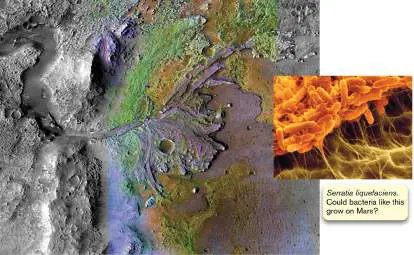
resemble a river delta, best explained by a model involving the flow of liquid water. Green indicates claylike mineral deposits. Inset: Serratia liquefaciens, a Gram-negative bacterium that survives extreme conditions found on Mars.
NASA/JPL-CALTECH/MSSS/JHU-APL
SCIMAT/SCIENCE SOURCE
In one crater with flow patterns, in 2022 NASA’s Perseverence rover found organic molecules and sulfate minerals that could have been produced by ancient life. However, abiotic origin of these molecules cannot be ruled out.
If life once existed on Mars, what became of it? Two main possibilities are considered: Life developed and existed until the planet froze. Under this scenario, life originated much as it did on Earth, during a time of heavy bombardment from space and outgassing of nitrogen and carbon dioxide. Unfortunately, however, life failed to generate sufficient atmosphere for a greenhouse effect to sustain temperate conditions. No oxygenic organisms produced molecular oxygen and an ozone layer.
Life developed and still exists underground. In the absence of an ozone layer, the Martian surface is sterilized by cosmic radiation. Nevertheless, microbes may yet exist deep underground, similar to the endolithic prokaryotes on Earth or the subsurface brine communities of Antarctic lakes. Subsurface microbes are protected from cosmic radiation.
In 2018, a team of Italian astronomers reported radar evidence for liquid water beneath the ice cap of the Martian south pole. The team analyzed data from the Mars Advanced Radar for Subsurface and Ionosphere Sounding (MARSIS), an instrument on the Mars Express orbiter sent by the European Space Agency. The analysis indicates a large subglacial lake. The lake probably consists of perchlorate brine whose antifreeze property keeps the water liquid. On Earth, some microbes have been found to grow in such brines.
Do Biosignatures Indicate Life?
If microbes do exist on Mars, they should be detectable. But the detection of unknown life, even on Earth, remains a challenge. The advent of PCR sequence detection of species on the basis of ribosomal genes has revealed thousands of unknown species, most of which cannot be grown or recognized by other methods. Other species may well be missed if their rRNA sequences fail to amplify with our probes. On Mars, assuming life evolved independently of Earth life forms, we would have no way to define sequence probes for detection.
Instead, researchers try to define biosignatures, chemical and physical signs that only life could have formed. Most of the proposed biosignatures are based on types of evidence for life on Earth, either as fossils of ancient life (discussed in Chapter 17) or as signs of current life in extreme habitats. Proposed biosignatures include the following: Microfossils. The mineralization of microbial cells leads to the formation of structures that can be visualized under a microscope. The cell fossils must be sufficiently distinct to establish that no abiotic process could have formed them. Isotope ratios. Certain biochemical reactions preferentially use one isotope of an atom over another; for example, Rubisco, the key enzyme of carbon dioxide fixation, uses 12 C in preference to 13 C (discussed in Chapter 17). Thus, both photosynthetic and chemolithoautotrophic use of 12 C can decrease the 12 C/ 13 C ratio in subsequent carbonate deposits. Isotope ratios of nitrogen, oxygen, and sulfur are also used as biosignatures.
Mineral deposits. Certain mineral formations are observed to be caused only by microbial activity. For example, insoluble manganese oxides such as Mn 2 O 3 are almost always the result of microbial oxidation of reduced manganese (discussed in Chapter 14). Reduced manganese ions are very stable, and their abiotic oxidation rate is extremely slow.
Metabolic activity. Samples of soil can be incubated with radioactive tracer substances such as 14 CO and tested for
2
metabolic conversion or incorporation into biomass. It must be established that the conversion could not have occurred abiotically and that no organisms from Earth were present. Various kinds of evidence for life on Mars have been reported, such as possible microfossils within a Martian meteorite that landed in Antarctica. Metabolic activity was tested in samples obtained by the NASA Viking lander in 1975. As of this writing, however, no evidence has proved conclusive for active or past living microorganisms on Mars.
What kinds of microbes might survive on Mars? Terrestrial bacteria in extreme habitats suggest possibilities. For example, the halophilic archaeon Halorubrum lacusprofundi, isolated from Deep Lake, Antarctica, grows in high salt at temperatures below 0°C. Other Haloarchaea, such as Haloarcula argentinensis, grow in solutions of up to 0.5-M perchlorate, a powerful oxidant found in high concentration on Mars. The Gram-negative bacterium Serratia liquefaciens (Fig. 22.32, inset) was shown to survive subfreezing temperatures (−50°C), ultraviolet exposure, and low atmospheric pressures—all conditions comparable to those found on Mars.
Could Mars Be Terraformed to Support Earth Life?
If no life exists on Mars—or if it exists only in the form of microbes deep underground—should we consider human intervention, or terraforming, to make Mars habitable for life from Earth? Scenarios for terraforming, long explored in science fiction, are now receiving serious thought among space scientists. Terraforming Mars would require increasing the temperature and air pressure. The temperature of the atmosphere might be increased by release of greenhouse gases. In addition, sufficient carbon dioxide and nitrogen gases must be made available from the Mars surface rock. In principle, microbes from Earth could be seeded to grow and generate an atmosphere containing nitrogen, oxygen, and CO 2. The dilemmas and consequences of terraforming are depicted in the novel Red Mars (1993) by Kim Stanley Robinson. In favor of terraforming, it is argued that Mars offers enormous natural resources of potential benefit for humanity, especially as terrestrial resources are used up. Human settlements on Mars would be a major step forward for space exploration. On the other hand, it is argued that the planet Mars is a natural monument, a place with its own right to exist as such, and should be allowed to remain in its natural state for future generations to appreciate. As a practical matter, terraforming remains unfeasible for the near future. For example, the amount of chlorofluorocarbons required to raise Martian temperature is calculated to be 100 times greater than our global capacity to produce such substances.
Does Europa Have an Ocean?
Farther out in the solar system, surprising candidates for microbial life are the moons of Jupiter. In 2000, the Galileo space probe passed several of Jupiter’s moons, including Ganymede, Callisto, and Europa (Fig. 22.33). While their distance from the Sun results in extreme cold, these bodies receive extra heat from friction generated by tidal forces from the giant planet Jupiter. In the case of Europa, the tidal forces have been calculated to provide enough heat to liquefy water without boiling it off. Furthermore, measurement of Europa’s magnetic field suggests that its composition includes a dense iron core surrounded by 15% water. Most of the water must be locked in ice, but tidal heating could melt enough water for an underlying ocean of brine. On Earth, similar brine lakes beneath the ice of Antarctica harbor halophilic archaea that grow at −20°C.
FIGURE 22.33 ■ Jupiter’s moon Europa. Does life exist beneath Europa’s ice, in a salty sea?
NASA/DRL
If such oceans do exist, how could they support life without photosynthesis? Photosynthesis is impossible at Jupiter’s distance from the Sun. However, an alternative source of chemical energy might be the influx of charged particles accelerated in Jupiter’s magnetic field. Charged particles entering Europa’s ice can react with water to form hydrogen peroxide (H 2 O 2). The H 2 O 2 then breaks down, releasing molecular oxygen. Oxygen reaching the
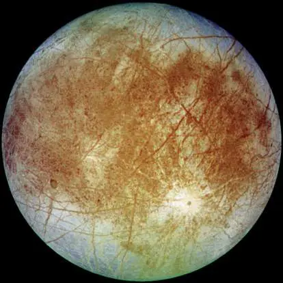
brine layer below could combine with electron donors from crustal vents and power metabolism. Alternatively, molecular hydrogen (H 2 ) could be generated from water ionized by decay of radioisotopes. A similar source of H 2 for life has been proposed to occur on Earth in rock strata several kilometers below the surface, where it may support lithotrophs. On Europa, the hydrogen could then combine with oxygen gas or other oxidants to power life. These schemes are highly speculative—but tantalizing enough to encourage future NASA missions to take a closer look at Europa and its sister moons.
Does Life Exist on Planets of Distant Stars?
The past decade of astronomy has seen an extraordinary growth in our knowledge of solar systems beyond our own. Now that we know that so many other stars possess planets, we can only wonder whether they also possess biospheres of life forms we would recognize.
In recent years, astronomers have found several thousand extrasolar planets orbiting distant stars, including some planets the size of Earth. Could we ever hope to detect signs of life on an extrasolar planet? A possible sign for detection is that light scattered by phototrophic microbes and plants exhibits a property called “circular polarization.” Circular polarization arises from substances that are homochiral; that is, present in only one of two mirror forms, such as the L and D forms of an amino acid. Homochirality is a strong biosignature, typical of proteins and metabolites. Remote sensing based on homochirality could help us assess habitat loss and other biospheric changes on Earth. If our telescope could detect light from distant planets, circular polarization might provide evidence of extraterrestrial life. The development of remote sensing for circular polarization is discussed in eResearch Activity 22.
Figure 22.34shows an infrared photograph through the Spitzer Space Telescope of nebula RCW-49, a gaseous cloud full of newborn stars. Recall from Chapter 17 that as stars form, they take up dust of supernovas that includes all the elements needed to form biomolecules. Spectroscopic observation of RCW-49 reveals stars surrounded by disks coalescing into planets. The planetary disks contain icy particles full of organic molecules such as methanol, glycine, and ethylene glycol, a reduced form of sugar. Could there be biospheres in the making?
FIGURE 22.34 ■ A stellar nursery. Nebula RCW-49 contains more than 300 newborn stars, from which NASA’s Spitzer Space

Telescope detected spectroscopic signals of common organic constituents of life (infrared photograph).
NASA
Whether life exists elsewhere or we are alone, we must remember that Earth is the only place we know of at this time that can support humans and the forms of life we require for our own survival. The survival of Earth’s entire biosphere depends on our microbial partners cycling key elements and acquiring energy to drive the food web. For the first time in history, human technology now rivals the ability of microbes to alter fundamental cycles of biogeochemistry. But to manage and moderate our alterations—for our own survival and that of the biosphere—our fate still depends on the microbes.
To Summarize
Astrobiology is the study of life in the universe, including possible habitats outside Earth.
Mars is the planet whose geology most closely resembles that of Earth. Geological features strongly support the past existence of flowing water, a prerequisite for microbial life.
The search for extraterrestrial life is based on methods similar to those used to seek early life on Earth. Evidence includes chemical and physical biosignatures, isotope ratios, microfossils, and metabolic activity.
Terrestrial extremophile microbes are found that survive some of the conditions found on Mars.
Haloarchaea survive high salt and perchlorate, while certain bacteria survive ultraviolet exposure and low atmospheric pressures.
Jupiter’s moon Europa is proposed as another possible site for life. Europa is bathed in a sea of brine similar to terrestrial habitats for halophiles.
Remote sensing of circular polarization might detect biosignatures of life on distant planets.
Glossary
biosignature Also called biological signature. A type of chemical believed to be formed only by specific life processes.
terraforming The idea of transforming the environment of another planet to make it suitable for life from Earth.
eResearch Activity 22
Look Up: Can We See Life on Distant Planets?
Humans have long dreamed of exploring life on other planets. Few of us will have the opportunity to visit another planet such as Mars, let alone planets elsewhere in our galaxy. But now we can visualize certain extrasolar planets (exoplanets) by a telescope such as the James Webb Space Telescope, deployed in orbit by NASA in 2022. Could light rays reflected by a distant planet carry a kind of information that reveals life?
Brice Demory and Lucas Patty at the University of Bern, Switzerland, are devising methods that someday might be able to see life on distant worlds (Fig. ERA 22.1 ). Remote sensing of life would have extraordinary consequences for our view of the universe. Even if that prospect is far off, the methods invented as first steps might find use closer to home, such as assessing the state of Earth’s global biosphere.
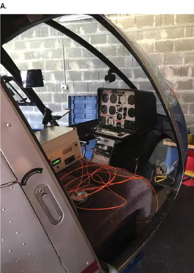
FIGURE ERA 22.1 ■ Detecting biosignatures remotely. A. The airborne FlyPol instrument measures the circular polarization

of light reflected by a landscape. B. Lucas Patty at University of Bern, Switzerland, develops devices for remote sensing of life.
COURTESY LUCAS PATTY
COURTESY LUCAS PATTY
The method Demory’s team developed uses circular polarization of light (Fig. ERA 22.2A ). Circular polarization means that light’s alternating waveforms of electrical and magnetic field vectors propagate not in a flat line, but with a twist. Light waves reflected by microbes and other living organisms are circularly polarized because biological material consists of molecules that are chiral; that is, right-or left-handed mirror forms. Recall that the great French microbiologist Louis Pasteur first discovered that molecules can have a handedness—and that molecules produced by microbes, such as yeast fermenting grapes, could be made entirely in one mirror form (see Chapter 1). That is because most of life’s chemical reactions are catalyzed by enzymes, which exist in one mirror form and generate only products in one mirror form. So chirality is a fundamental property that distinguishes biomass (material made by life) from abiotic materials.
FIGURE ERA 22.2 ■ Circularly polarized light is reflected by biological landscape features. A. Circular polarization of a
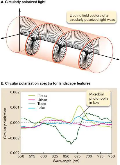
light wave, with right-handed twist of the electric field vectors. B. Circular polarization signals from various landscape features. The researchers designed an electronic detector that measures the fractional polarization of light; that is, of all the light radiation detected, what fraction is polarized. Extremely small fractions were detectable. The degree of polarization varies with wavelength, so measurement is taken across the spectrum (spectropolarimetry). The instrument for spectropolarimetry was mounted on a helicopter and flown at 1.7 km above various regions of terrain in the Swiss Alps. The spectrum of light reflectance was measured above landscape features such as grass, urban area (roofs and walls), forest trees, and lake water (Fig. ERA 22.2B ). Positive and negative numbers indicate the two opposite directions of circular polarization. In Figure ERA 22.2B , grass and trees show negative and positive signals around the wavelength of red light, 680 nm. This finding is consistent with the known polarization of light reflected by chlorophyll arrays within chloroplasts, where the regular packing of the chlorophyll magnifies the light polarization. Lake water also shows a distinct band of polarization, which is consistent with the presence of chloroplasts in algae, even though they are well dispersed in the water. Thus, even planktonic microbial phototrophs can be detected remotely. By contrast, regions of buildings close together without vegetation (labeled “Urban” in Fig. ERA 22.2B ) show no polarization signal.
How can remote sensing be used in the future? While many technical challenges remain, we can likely use spectropolarimetry to assess various features of ecosystems on Earth. For example, the polarization fraction declines with loss of chlorophyll organization, so it may serve as a measure of health of a forest canopy. In water bodies, circular polarization could indicate algal blooms, coral reefs, and the loss of viable chlorophyll content due to acidification or oil spills. Even if we cannot yet find life on exoplanets, we can still look up and gain data to help save our home biosphere.
Further Exploration
How could airborne remote sensing of circular polarization help us assess climate change on Earth? What further advances would be needed to detect life on other planets? What challenges would we need to overcome?
Patty, C. H. Lucas, J. G. Kuhn, Petar H. Lambrev, Stefano Spadaccia, H.
Jens Hoeijmakers, et al. 2021. Biosignatures of the Earth. I. Airborne
spectropolarimetric detection of photosynthetic life. Astronomy & Astrophysics 651
:A68.
CHAPTER REVIEW
Review Questions
1. Identify the major sources and sinks of carbon, nitrogen, and sulfur. Which sources recycle rapidly, and why? 2. Explain how the carbon cycle differs in oxygenated and anoxic environments.
3. Explain two different chemical methods of measuring the environmental levels of carbon and nitrogen.
4. Outline the hydrologic cycle. Explain the role of biochemical oxygen demand (BOD) in water quality and how it may be perturbed by human pollution.
5. Outline the functions of a wastewater treatment plant. Include the phases of primary, secondary, and tertiary treatment. Explain the roles of microbes in these phases of water treatment.
6. Outline the main transformations of the nitrogen cycle. Which reactions are carried out only by microbes?
7. Outline the main transformations of the sulfur cycle. Which features are comparable to the nitrogen cycle, and which are unique to the sulfur cycle?
8. For the iron cycle, explain aerobic and anaerobic processes of microbial transformation. Explain how microbial iron transformation may be linked to sulfur transformation.
9. Explain how bacteria may convert metals to toxic forms. Alternatively, explain how bacteria may detoxify metal-polluted sediment.
10. Explain the sources of microbes in the human-built environment. How are humans affected by members of the built-environment microbiome?
11. Offer several arguments for and against the existence of life on planets beyond Earth.
Thought Questions
1. How does influx of nitrogen-rich fertilizers to soil ecosystems increase the rate of CO 2 efflux from wetlands?
2. In the past 50 years, most of the wetlands off the coast of Louisiana have been destroyed. How is wetland destruction related to formation of the dead zone in the Gulf of Mexico? How could the dead zone be revived, and why would the cost of restoration be projected to be billions of dollars?
3. What nutrients are limiting in the marine benthos, and why?
Key Terms
abiotic (910)
aerosol (942)
air recirculation (944)
ammonification (931)
anammox reaction (932)
assimilatory nitrate reduction (931) biochemical oxygen demand (BOD) (921) biogeochemical cycle (910) biogeochemistry (910)
biological carbon pump (914) biosignature (947)
biotic (910)
built environment (910)
constructed wetland (927) dead zone (922)
denitrification (931)
dissimilatory nitrate reduction (931) floc (924)
fossil fuel (917)
geomicrobiology (910)
greenhouse effect (910)
high-efficiency particulate air filter (HEPA filter) (944) hydrologic cycle (921)
hypoxia (922)
leading indicator (926)
mesocosm (913)
nitrification (930)
nitrifier (930)
nitrogen fixation (929)
oxygen minimum zone (OMZ) (922) radiative forcing (916)
reservoir (911)
resource colimitation (938) siderophore (937)
sink (911)
sludge (923)
source (911)
terraforming (947)
ventilation (943)
wastewater treatment (923) water cycle (921)
zone of hypoxia (922)
Recommended Reading
Al-Shayeb, Basem, Marie C. Schoelmerich, Jacob West-Roberts, Luis E. Valentin-Alvarado, Rohan Sachdeva, et al. 2022. Borgs are giant genetic elements with potential to expand metabolic capacity. Nature. doi:10.1038/s41586-022-05256-1 Canfield, Donald E., Alexander N. Glazer, and Paul G. Falkowski. 2010. The evolution and future of Earth’s nitrogen cycle. Science 330 :192–193.
Clemmensen, Karina E., Adam Bahr, Otso Ovaskainen, Anders Dahlberg, Alf Ekblad, et al. 2013. Roots and associated fungi drive long-term carbon sequestration in boreal forest. Science 339 :1615–1618.
Conway Morris, Andrew, Katherine Sharrocks, Rachel Bousfield, Leanne Kermack, Mailis Maes, et al. 2022. The removal of airborne severe acute respiratory syndrome coronavirus 2 (SARS-CoV-2) and other microbial bioaerosols by air filtration on coronavirus disease 2019 (COVID-19) surge units. Clinical Infectious Diseases 75 :e97–e101.
Gilbert, Jack A., and Brent Stephens. 2018. Microbiology of the built environment. Nature Reviews. Microbiology 16 :661–670. Heinz, Jacob, Janosch Schirmack, Alessandro Airo, Samuel P. Kounaves, and Dirk Schulze-Makuch. 2018. Enhanced microbial survivability in subzero brines. Astrobiology 18 :1171– 1180.
Hutchins, David A., and Douglas G. Capone. 2022. The marine nitrogen cycle: New developments and global change. Nature Reviews. Microbiology 20 :1–14.
Karlusich, Pierella, Juan José, Chris Bowler, and Haimanti Biswas. 2021. Carbon dioxide concentration mechanisms in natural populations of marine diatoms: Insights from Tara Oceans. Frontiers in Plant Science 12 :659.
Marlow, Jeffrey J., Daniel Hoer, Sean P. Jungbluth, Linda M. Reynard, et al. 2021. Carbonate-hosted microbial communities are prolific and pervasive methane oxidizers at geologically diverse marine methane seep sites. Proceedings of the National Academy of Sciences USA 118 :e2006857118.
Melton, Emily D., Elizabeth D. Swanner, Sebastian Behrens, Caroline Schmidt, and Andreas Kappler. 2014. The interplay of microbially mediated and abiotic reactions in the biogeochemical Fe cycle. Nature Reviews. Microbiology 12 :797– 808.
Montzka, S. A., E. J. Dlugokencky, and J. H. Butler. 2011. Non-CO 2 greenhouse gases and climate change. Nature 476 :43–50. Salese, Francesco, Monica Pondrelli, Alice Neeseman, Gene Schmidt, and Gian G. Ori. 2019. Geological evidence of planet-wide groundwater system on Mars. Journal of Geophysical Research. Planets 124: 374–395.
Vuitton, Dominique Angèle, and Jean-Charles Dalphin. 2017. From farming to engineering: The microbiota and allergic diseases. Engineering 3 :98–109.
Woodcroft, Ben J., Caitlin M. Singleton, Joel A. Boyd, Paul N. Evans, Joanne B. Emerson, et al. 2018. Genome-centric view of carbon processing in thawing permafrost. Nature 560 :49–54. Wright, Jody J., Kishori M. Konwar, and Steven J. Hallam. 2012 . Microbial ecology of expanding oxygen minimum zones. Nature 10 :381–394.
Zhou, Zhuo, Cui-jing Zhang, Peng-Fei Liu, Lin Fu, Rafael Laso-Pérez, et al. 2022. Non-syntrophic methanogenic hydrocarbon degradation by an archaeal species. Nature 601:257–262.
Glossary
built environment Buildings and other human-built constructs that humans inhabit or use for work and recreation.
abiotic Produced without living organisms; occurring in the absence of life.
biotic Caused by living organisms.
biogeochemical cycle The recycling of elements needed for life (such as carbon or nitrogen) through the biotic and abiotic components of the biosphere.
biogeochemistry Also called geomicrobiology. The metabolic interactions of microbial communities with the abiotic (mineral) components of their ecosystems.
geomicrobiology See biogeochemistry .
greenhouse effect The trapping of solar radiation heat in the atmosphere by CO 2; a cause of global warming.
reservoir 1. The major part of the biosphere that contains a significant amount of an element needed for life. 2. An organism that maintains a virus or bacterial pathogen in an area by serving as a high-titer host.
source A part of the biosphere that stores a significant quantity of a given element; may be biotic (as in tree biomass, a source of carbon) or abiotic (as in carbonate rock).
sink A part of the biosphere that can receive or assimilate significant quantities of an element; may be biotic (as in plants fixing carbon) or abiotic (as in the ocean absorbing carbon dioxide). mesocosm A small, controlled model ecosystem.
biological carbon pump The fixation of carbon dioxide by phototrophs and gravitational settling of biomass particles within the oceans.
radiative forcing The increase in warming of Earth’s atmosphere (in watts per square meter) associated with a particular climate factor, which is calculated as the difference between the sunlight energy absorbed by Earth and the energy radiated out to space. fossil fuel Ancient organismal remains that have been converted to hydrocarbons (petroleum and natural gas) or sedimentary rock (coal) through microbial digestion followed by reduction under high pressure underground. Fossil fuels are extracted and burned by humans for energy.
hydrologic cycle Also called water cycle. The cyclic exchange of water between atmospheric water vapor and Earth’s bodies of liquid water. water cycle See hydrologic cycle .
biochemical oxygen demand (BOD)
Also called biological oxygen demand. The amount of oxygen removed from an environment by aerobic respiration.
oxygen minimum zone (OMZ)
The region of the marine water column in which oxygen is depleted by respiration; usually at a mid level, between the aerated upper water and the deeper oxygenated water where organic food is scarce.
dead zone Also called zone of hypoxia. An anoxic region of an ocean or freshwater system, devoid of most fish and invertebrates. zone of hypoxia See dead zone .
hypoxia A state of lower-than-normal oxygen concentration.
wastewater treatment A series of wastewater transformations designed to lower biological oxygen demand and eliminate human pathogens before water is returned to local rivers.
sludge The solid products of wastewater treatment.
floc Also called activated sludge. Particulate matter formed by clumps of microbes during wastewater treatment.
leading indicator In epidemiology, a signal that appears ahead of a trend such as increasing cases of a disease.
constructed wetland A built environment designed to provide environmental services comparable to those of natural wetlands.
nitrogen fixation The ability of some prokaryotes to reduce inorganic diatomic nitrogen gas (N) to two ammonium ions (2NH +).
2 4
nitrifier An organism that converts reduced nitrogen compounds to nitrite or nitrate.
nitrification The oxidation of reduced nitrogen compounds to nitrite or nitrate.
assimilatory nitrate reduction The uptake of nitrate and reduction to NH + by plants, fungi,
4
archaea, and bacteria for use in biosynthetic pathways. ammonification The generation of ammonia from organic nitrogen.
denitrification Also called dissimilatory nitrate reduction. Energy-yielding metabolism in which nitrate (NO −) is reduced to nitrite (NO
3 2
−), diatomic nitrogen (N), and in some cases ammonia (NH
2 3
).
dissimilatory nitrate reduction See denitrification .
anammox reaction The anaerobic oxidation of ammonium to nitrogen gas, using nitrite as electron acceptor; yields energy.
siderophore A high-affinity iron-binding protein used to scavenge iron from the environment and deliver it to a siderophore-producing organism.
resource colimitation A situation in which a population size is limited by the lack of two different resources, such as nitrogen and phosphorus. aerosol Water droplets suspended in air, of size 5 μm or smaller. The term also refers to suspension of dust or volcanic ash. ventilation In building maintenance, the exchange of indoor air with fresh outdoor air.
air recirculation The passage of air through a filter followed by return to the source.
high-efficiency particulate air filter (HEPA filter)
A medical-grade filter that is certified by government standards to remove at least 99.97% of all airborne particles and droplets of diameter 0.3 μm or larger.
biosignature Also called biological signature. A type of chemical believed to be formed only by specific life processes.
terraforming The idea of transforming the environment of another planet to make it suitable for life from Earth.