PHYS 1164 · Physics 2 Lab

Charge can't be measured directly, so you get it from a force: charge two plates, hold them close and parallel, and let the IOLab force sensor read the electric push between them. A parallel-plate model then converts that force into the charge.

⚠️ The #1 rule: the charged plates must be insulators (plastic lid, styrofoam or plastic plate). Aluminum foil is a conductor — it won't hold charge by rubbing and drains the moment you touch it, so a foil plate reads ~0 force. Use two insulating plates, same size, handled by the edges only.

The model

For two parallel charged plates: F = 2k·Q² / A → Q = √( F · A / (2k) ) (F = measured force in N, A = plate area in m², k = 9×10⁹). Compare force close vs far — the model predicts it's roughly constant. A sensible result is ~0.01–1 µC.

📐

Illustrated setup guide — open →

Foolproof step-by-step with labeled SVG diagrams & force arrows: build 2 insulator plates → measure area A → calibrate the force sensor → charge hard → read the force close vs far → calculate Q. Includes a foolproofing checklist + the High-Gain foil backup.

Open →

Build 2 insulating plates the same size; tape a handle on each; measure the area A (m²).
IOLab → select the Force sensor and CALIBRATE it (zero at rest). Mount plate #1 on the force probe.
Charge both plates hard on carpet/wool; handle by the edges only.
Record → 2 s baseline → bring plate #2 parallel, CLOSE (~2–3 cm), hold still → read the Mean force (N).
Repeat at FAR (~8–10 cm); do 3–5 trials each, recharging every time.
Punch F & A into the calculator/formula → Q = √(F·A/2k), average, uncertainty → paste into the report.

🔁 Two alternatives if the force is too tiny to read: (A) High-Gain foil sensor — charge a plastic lid, sense with foil on G+/G−→GND, read the induced voltage (needs the handout's V→Q calibration; confirm your instructor accepts it). (B) Balloon balance — the balloon guide → and its report/calculator below. Both are in the setup guide.

🌵 Static tips: dry hands + dry room · charge hard · work fast (charge leaks in seconds) · never touch the charged faces · calibrate the force sensor first.

🗺️ Lab 3 — Equipotential Surfaces

Map the "voltage contour lines" around two electrodes. Put salt water in a styrofoam plate, drive 3.3 V across it between two pennies (one on the IOLab DAC, one on GND), and probe the water with a clip on A7 to find points at the same voltage — those points trace an equipotential line.

The idea

An equipotential line connects points of equal voltage. Lines never cross (a point can't have two voltages), and electric field lines cross them at 90°. You'll map a symmetric and an asymmetric penny arrangement and compare the patterns — like reading a topographic map.

📐

Illustrated setup guide — open →

Beginner step-by-step with SVG diagrams: salt-water plate + 2 pennies wired to DAC/GND, the A7 probe, the software config (3.3 V + A7 + digital meter), symmetric vs asymmetric mapping, connect + label the lines, and the failure-mode checklist.

Open →

~¼" salt water in a styrofoam plate (tap water + stir in salt).
Alligator clip + penny on each of two opposite sides (edge submerged) → one to DAC, one to GND. A third clip (no penny) → A7 = probe.
Software: gear → Chart Display → check Output Configuration → DAC = 3.3 V → turn on Analog 7 → click the chart title to collapse it into a digital voltage meter.
Probe the water; find several points at the same voltage; mark each with a shallow dent (don't puncture!). Repeat at other voltages.
Empty + dry, connect same-voltage dots with a sharpie, label each line's voltage.
Do two plates — symmetric & asymmetric — and photograph both for the report.

⚠️ The "calibration" for this lab = setting DAC = 3.3 V (with Output Configuration checked) + turning on A7 + clicking into meter mode. No reading? Check those. Too weak a gradient? Add more salt & submerge the penny edges. Keep the two pennies from touching (short).

🔌 IOLab setup (web version — no install)

Put 2× AA batteries in the IOLab and turn it on.
Plug the USB dongle into the laptop.
Open Chrome → iolab.science/iolabweb (works without installing anything).
Click Connect → when the browser asks, select the dongle and Allow.
Not found? Turn the device OFF, hold + while turning it back ON (Discovery Mode) → Pair.
Test: Record → wiggle it → if the graph moves, you're connected. ✅

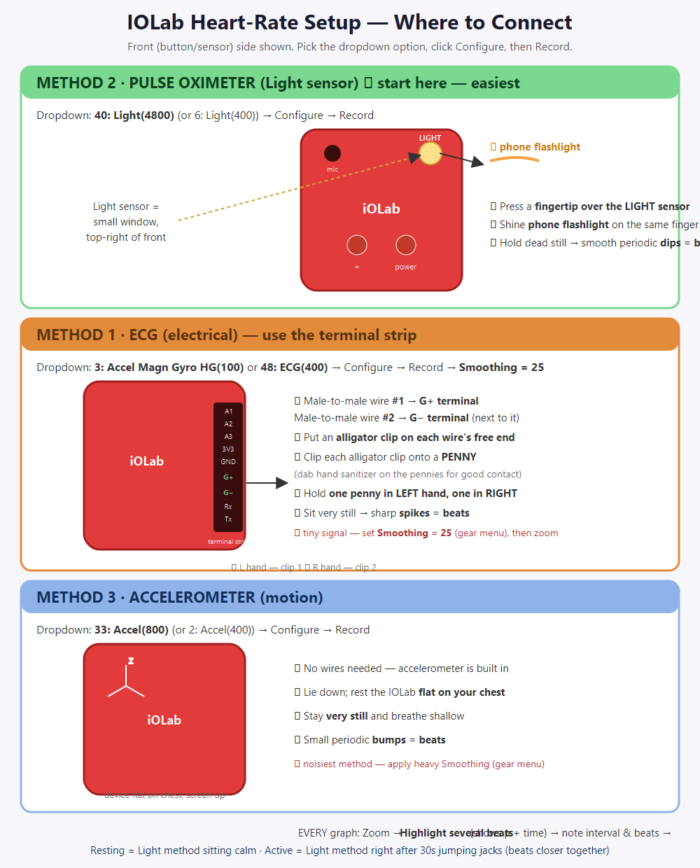
⚠️ Used device (eBay): no license/registration needed — the software is free. Just make sure the dongle is paired to your device.

❤️ The 5 heart-rate graphs (3 methods + resting/active)

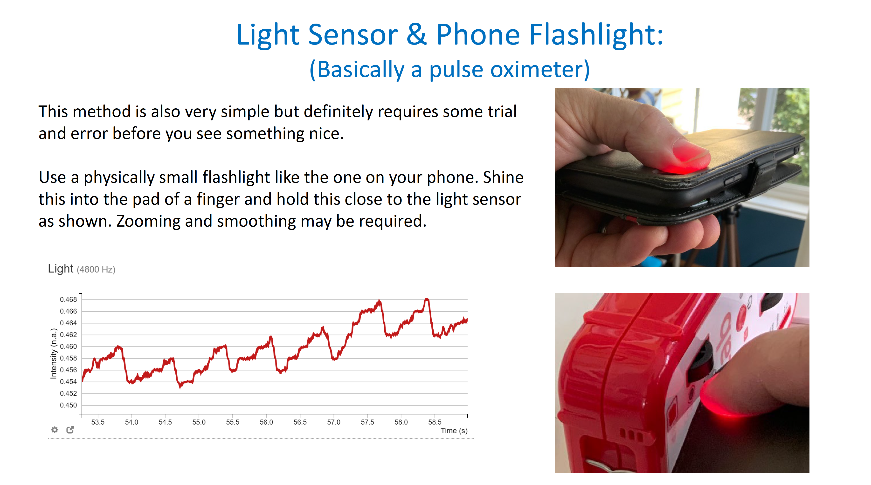
Method 2 · Pulse Oximeter (Light sensor) — ⭐ start here, easiest

Dropdown: 40: Light(4800) or 6: Light(400) → Configure → Record. Shine your phone flashlight into the pad of a finger and press that finger against the light sensor. Zoom + smooth. Each dip = a beat.

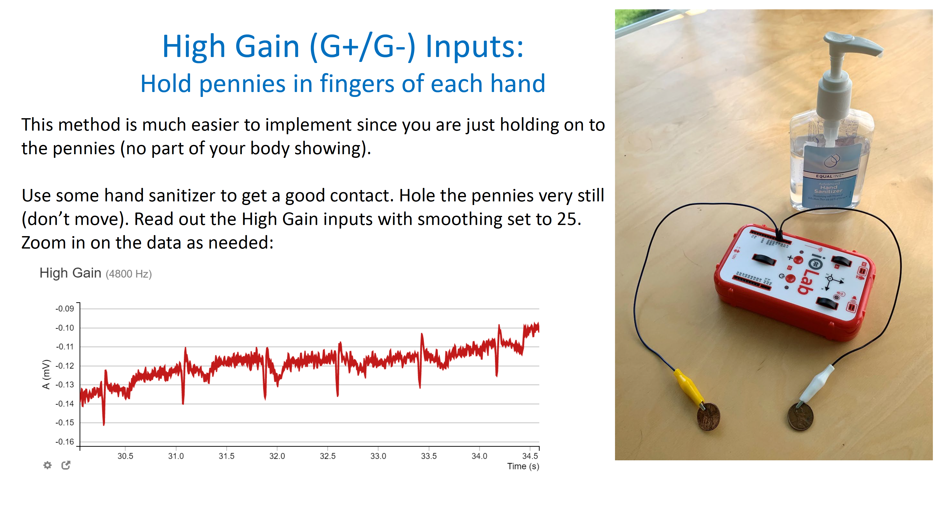
Method 1 · ECG (electrical / high-gain) — the penny trick

Dropdown: 48: ECG(400) or the HG combo → Configure → Record → Smoothing = 25. Wire #1 → G+ terminal, wire #2 → G− terminal; alligator clip on each free end; clip each to a penny (dab hand sanitizer for contact); hold one penny in each hand, very still. Sharp spikes = beats.

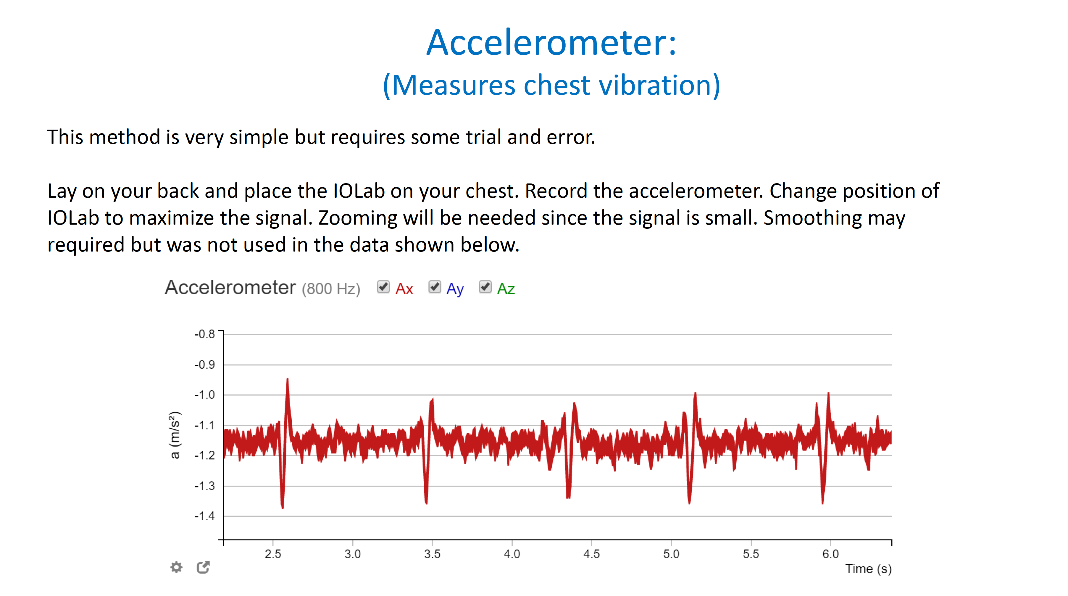
Method 3 · Accelerometer (motion)

Dropdown: 33: Accel(800) or 2: Accel(400) → Configure → Record. No wires — rest the IOLab flat on your chest, lie very still, apply heavy smoothing. Small bumps = beats.

Graphs 4 & 5 · Resting vs Active

Use the light sensor both times. Record resting (sitting calm), then do ~30 s jumping jacks and immediately record active — beats will be spaced closer together (faster).

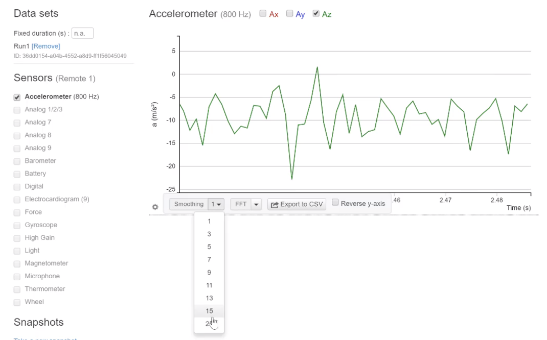
How to smooth noisy data

Every graph: zoom → Highlight several consecutive beats (shows μ + time span) → note interval & beats → Win+Shift+S screenshot (no phone photos!) → paste into the report → enter numbers in the BPM calculator.

📊 Lab 0 — Intro to Excel (reference)

Data: Distance/Time of a moving cart. Speed = d/t. Scatter (Time = x, Distance = y), linear trendline.

Key results (to check your own work)

Speeds: 0.52, 0.79, 0.97, 1.00, 1.10 m/s
Mean speed 0.88 · Sample SD (STDEV.S) 0.23
Toy-car times mean 4.90 s · Population SD (STDEV.P) 0.14 s (= error bar value)
Trendline y = 1.51x − 2.03 · R² ≈ 0.997
Predict at 6.0 s → ≈ 7.03 m

Wrap-up answers A–I

A Speed is a calculated quantity (from measured d & t) — keep measured vs calculated separate.
B Slope = speed/velocity (rate of change of distance with time).
C y-intercept = distance at t=0 (initial position); slightly negative = small offset.
D R² near 1 = strong linear fit (variables highly correlated).
E Graph Y (professional: title, labeled axes w/ units, trendline, equation, R²).
F y = 1.51(6.0) − 2.03 ≈ 7.03 m.
G The (3.5 s, 3.4 m) point is farthest — random measurement error.
H Error bars ±0.14 s ≈ 3% of 4.90 s → fairly precise.
I (1.10 − 0.88)/0.23 ≈ 1.0 standard deviation.

✅ Quiz answers

Pre-lab 0.1 (IOLab + Excel videos)

iOLab purpose → collect & send data to a computer for real-time analysis
iOLab lets students → explore experiments independently & understand science broadly
Scatter plot → highlight data → Insert → Scatter Plot
Label axes → ensures accurate data interpretation
Excel version → Windows desktop version
Professional graph → titles for graph & axes
Trendline purpose → identify/describe the relationship between variables

Lab 1 pre-lab video quiz

Heart contracts all at once → False (coordinated sequence: atria then ventricles)
Camera detects heart rate → by tiny color changes in the skin over time
Accelerometer chip replaces ball-and-spring with → a comb-like silicon structure with flexible supports
Smartphone accelerometer main function → detect orientation and motion
Large error bars indicate → high uncertainty

Lab 0 post-lab assessment

Slope of trendline → relationship between distance and time (= speed)
Copy formula down → drag the fill handle (bottom-right square)
Objective of Excel lab → input, organize, analyze, visualize experimental data
Independent variable axis → the x-axis
Average function → =AVERAGE

⚠️ A timer logs whether you actually watched the videos (used for grade rounding) — let them play while you answer.

📦 PHYS 1164 take-home kit (provided — return at end)

You don't buy these; you're accountable for returning them. For Lab 1 you only need the IOLab, dongle, 2× AA, your phone, and — from the kit — 2 male-to-male wires + alligator clips (ECG method).

Item	Qty	Used for
Alligator clips	5	ECG leads (clip to pennies)
Male-to-male wires	2	ECG → G+/G− terminals
Breadboard + resistors (100/1k/10k Ω)	—	Ohm's law / RC circuits (later)
Diode	1	Circuits (later)
Capacitors (22 µF, 220 µF)	2	RC circuits (later)
Hanging magnet + copper wire	—	Induction / magnetism (later)
Polarizer film ×2, ruler, protractor	—	Optics (later)
Balloons ×3	3	Electrostatics (later)
4× AA + battery holder	—	Circuit power (later)